
Online publication date 14 Sep 2026
Investigation on the Structural Stability of Scale-down and Prototype Francis Hydro Turbine Models in the Range of Flexible Operation

Copyright © 2026 by the New & Renewable Energy
This is an Open Access article distributed under the terms of the Creative Commons Attribution Non-Commercial License (http://creativecommons.org/licenses/by-nc/4.0) which permits unrestricted non-commercial use, distribution, and reproduction in any medium, provided the original work is properly cited.
Abstract
Hydraulic turbines, essential for making accurate predictions of structural behavior under varying hydraulic loads, are increasingly operated under flexible conditions to support modern electricity grids. This study presents a comparative fluid-structure interaction (FSI) analysis of scaled-down and full-scale prototype Francis turbine models over a wide range of unit discharges representative of flexible operation. High-fidelity computational fluid dynamics (CFD) simulations capture the evolution of internal flow structures from part-load vortex-rope behavior to overload trailing-edge separation, whereas mapped transient pressure fields enable the structural evaluation of equivalent stress and total deformation. The results showed that the hydraulic performance improved toward the best efficiency point, whereas part-load conditions exhibited a strong vortex region and eddies in the blade passage. The prototype experienced significantly higher stress (100–120 MPa) and deformation (0.44–0.50 mm) than the scale-down model (<20 MPa, <0.01 mm). Based on the normalized results, the similarity between the scaled-down and prototype runners was most consistent with hydraulic performance, whereas pronounced deviations occurred in the structural analysis. This behavior demonstrates that scaled-down model predictions cannot be directly extrapolated to full-scale without accounting for scale-dependent structural effects, thereby emphasizing the importance of an integrated FSI analysis in evaluating runner stability across flexible operating regimes.
Keywords:
Francis hydro turbine, Flexible operation, FSI analysis, Deformation, Scale-down model, Prototype, Structural stability키워드:
프란시스 수차, 유연화 운전, 유체-구조 연성해석, 변형, 실물 모형, 축소 모형, 구조안정성1. Introduction
Hydropower remains one of the most reliable and controllable renewable energy sources, providing essential grid‑balancing services as modern power systems increasingly incorporate variable renewable energy.[1,2] As a consequence, hydropower units are now required to operate under a wide range of flexible operating conditions, including part‑load, overload, spinning reserve, and rapid transient events. These conditions significantly increase unsteady hydraulic phenomena in turbines, often leading to flow instabilities, vibration, and reduced structural lifetime.[3,4]
During part‑load operation, Francis and pump‑turbines frequently develop strong swirling flow in the draft tube, resulting in the formation of a vortex rope. This large‑scale structure induces low‑frequency pressure pulsations that can propagate upstream and interact with the hydraulic system.[5,6] Experimental and numerical studies have shown that vortex rope-induced oscillations significantly affect runner and guide vane loading, sometimes generating damaging dynamic interactions.[7,8] Conversely, under overload conditions, strong trailing edge flow separation leads to vortex shedding and high‑frequency fluctuations that contribute to blade fatigue and structural degradation.[9~11]
Scale‑model testing remains a fundamental tool for turbine design and performance assessment; however, model-to-prototype translation is challenging due to unsteady flow phenomena. Factors such as Reynolds number effects, surface roughness, turbulence scaling, and cavitation behavior introduce discrepancies between model and full‑scale behavior.[12,13] Studies comparing prototype and model pressure pulsations confirm that dynamic similarity is often incomplete, especially under off‑design operating condition.[14] These limitations highlight the need for high‑fidelity numerical methods to supplement model testing and support extrapolation to prototype behavior.[15,16] Recent advancements in Computational Fluid Dynamics (CFD) allow detailed resolution of three‑dimensional unsteady flows in hydraulic turbines. While RANS models such as SST κ―ω remain widely used for steady and moderately unsteady predictions,[17] more advanced methods, including Scale Adaptive Simulation SST, Large Eddy Simulation (LES), and Detached Eddy Simulation (DES), provide an accurate representation of complex flow structures such as draft tube swirl, vortex rope dynamics, and turbulent shedding.[18~20] Accurate simulations require careful mesh refinement, timestep selection, and uncertainty quantification procedures as recommended in CFD guidelines.[21,22] Because flow‑induced pressure pulsations directly excite turbine structural components, Fluid–Structure Interaction (FSI) approaches are essential for evaluating vibration response, stress distribution, and fatigue life. One‑way coupled CFD–FEA workflows have proven effective for transferring transient pressure fields from CFD solvers to structural finite‑element models.[23,24] Previous studies show that runner blades experience stress concentration zones—especially near hub and shroud junctions—and that these stresses amplify substantially when hydrodynamic excitation frequencies approach structural natural frequencies.[25,26] These findings emphasize the need for integrated FSI analysis when assessing turbine operation under flexible grid conditions.[27]
Characterizing the frequency content of unsteady hydraulic excitation requires advanced spectral analysis techniques such as the FFT, Welch averaging, and windowing methods.[28~30] ASME PTC 18 and ISO 9906 establish accepted methodologies for performance evaluation and pressure pulsation measurement in hydraulic turbines.[31,32] Structural dynamic analysis must also account for centrifugal stiffening and rotation‑induced modal shifts, which significantly influence runner vibrational behavior.[33~35] Cavitation, which becomes more prevalent in off‑design operating regimes, can alter local pressure distributions and accelerate erosion, adding complexity to both hydraulic and structural performance assessments.[36,37] Despite advances in understanding unsteady flow physics and structural dynamics, comprehensive FSI investigations comparing scale‑model and prototype turbines across the entire flexible operating range remain limited. The prior studies examine isolated components or specific operating points, leaving important questions regarding scaling laws, dynamic amplification, and load transfer mechanisms unresolved.[4,14] Therefore, a unified multi‑scale FSI framework is essential to accurately assess how unsteady hydrodynamic loads translate into prototype‑level structural responses.
The key objectives are to characterize unsteady flow behavior across varied flexible operational regimes, quantify fluid pressure to the finite-element structural models, compare stress and deformation between scale and prototype, and identify scaling effects governing flow–structure interactions. The study resolves the critical challenge of ensuring the structural stability of the Francis hydro turbine in the scale-down and prototype models in the range of flexible operation.
2. Modeling of Francis Turbine Model
The Francis turbine is widely used in medium to high-head hydroelectric plants, offering reliable and sustainable energy generation. The specifications of the Francis hydro turbine are shown in Table 1, which were calculated using Eqs. (1)-(4).
| (1) |
| (2) |
| (3) |
| (4) |

Specification of Francis hydro turbine model
The specific speeds of the Francis hydro turbine are 147 [min-1, kW, m] and 146 [min-1, kW, m] for the prototype and the scale-down model, respectively. This minor deviation (<1%) arises from numerical rounding and geometric scaling effect during model design. The difference is within an acceptable tolerance and does not affect hydraulic similarity. The reference diameter ratio between the prototype and scale-down model is 7.14, and the Francis hydro turbine is designed accordingly. Fig. 1 shows the 3D modeling of the Francis hydro turbine scale-down model, which consists of a spiral casing, a stay vane, a guide vane, a runner, and a draft tube.
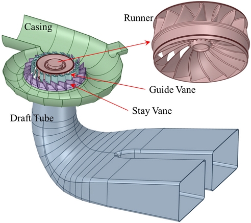
3D modeling of Francis hydro turbine scale-down model
3. Numerical Methodology
The computational domain of the Francis hydro turbine consists of the spiral casing, stay vanes, guide vanes, runner, and draft tube, as shown in Fig. 2. Each component was discretized independently to ensure optimal control of mesh quality and interface connectivity. A hexahedral dominant grid topology was generated using ANSYS ICEM 2024R2, providing high accuracy in capturing boundary‑layer gradients and maintaining low numerical dissipation in regions with strong streamline curvature. The inlet casing and stay/guide vane passages were meshed with structured multi‑block grids, while the runner utilized an O‑grid strategy around blade surfaces to accurately reproduce pressure gradients at the leading edge (LE) and trailing edge (TE). The draft tube, characterized by strong swirling and decelerating flow, was also discretized using structured blocks to minimize interpolation errors. Three systematically refined meshes (G1, G2, and G3) were generated to assess grid‑induced numerical uncertainty[21]. The total cell counts for the prototype case were 19.20×10⁶, 9.26×10⁶, and 4.97×10⁶, with y+ values for the runner domain of 18, 24, and 54, respectively. The detailed results for the grid convergence test are shown in Table 2. The simulation on the finest grid G1 with medium grid G2 has discretization errors of 0.04%, 1.81%, and 0.03% for N11, Q11, and P11, respectively, confirming that the medium grid provides grid‑independent results while maintaining computational efficiency.
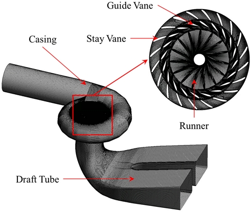
Numerical grids of Francis hydro turbine model components
Specification of Francis hydro turbine model
The incompressible, three‑dimensional Reynolds‑Averaged Navier–Stokes (RANS) equations were solved using the finite‑volume solver ANSYS CFX 2024R2. For steady‑state simulations, the Shear Stress Transport (SST) model was employed due to its superior performance in capturing adverse pressure gradients around blade surfaces[17]. To analyze unsteady flow behavior—including wake interaction, rotating stall, and draft‑tube swirl—the Scale‑Adaptive Simulation SST (SAS‑SST) model was applied. The numerical settings for the CFD analysis of the scale-down model are summarized in Table 3. A total pressure condition was imposed at the spiral‑casing inlet, while static pressure was prescribed at the draft‑tube outlet. All walls were treated as no‑slip with automatic wall functions.
Numerical settings of CFD analysis for Francis hydro turbine scale-down model
The structural analysis was performed using the linear dynamic equilibrium equation, as shown in Eq. (5).[38] The Rayleigh Damping was implemented as a linear combination of the mass and stiffness matrices. The damping coefficient α and β are dependent on the material properties.
| (5) |
| (6) |
The structural displacement x is obtained from Eq. (5), which can be used to obtain flow-induced stress σ in the Francis hydro turbine runner using Eq. (7).
| (7) |
The equivalent stress is defined by Eq. (8), with the maximum, middle, and minimum principal stresses adopted to assess the structural behaviour of the Francis turbine.
| (8) |
Pressure fields obtained from the CFD simulations were exported and mapped onto the structural finite‑element model of the Francis runner using a consistent nodal interpolation scheme to minimize projection errors, with data transfer performed through the direct coupling interface in ANSYS Workbench. During structural analysis, the runner hub was constrained through a fixed‑support boundary condition, while the operational rotational speed was applied as a centrifugal body load in combination with standard Earth gravity (9.806 m/s2). The pressure fields imported from the CFD calculations were applied as distributed loads across all blade surfaces to reproduce realistic hydraulic forcing.
Figure 3 shows the numerical settings for structural analysis. The structural domain was discretized using high-quality quadratic tetrahedral solid elements, and material properties representative of stainless steel commonly used in Francis turbine runners were assigned to capture accurate stiffness and stress behavior under coupled fluid–structure loading, as shown in Table 4.
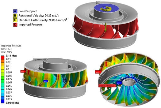
Numerical settings for FSI analysis of scale-down model
Material properties used for Francis hydro turbine runner[39]
4. Results and Discussion
4.1 Performance Curves of the scale-down model and the prototype
The guide vane opening controls the flow rate in the Francis hydro turbine model. CFD analysis predicted the flow rate for each guide vane opening. The unit speed (N11), unit discharge (Q11), and unit power (P11) are used to evaluate the performance of the Francis hydro turbine shown in Eqs. (2)-(4). The normalized efficiency (η11) compares the performance of the Francis hydro turbine and is calculated using Eq.(9).
| (9) |
Figure 4 presents the performance curves of the Francis hydro turbine derived from scale-down model experiments[40] and CFD simulations for both the prototype and the scale‑down model. The experimental and CFD analysis results indicated good agreement and justify the acceptance of the CFD analysis. The scale‑down model exhibits a smooth rise in unit efficiency with increasing Q11, reaching its maximum near Q11≈0.71, which corresponds to the numerically predicted best-efficiency point (BEP). The prototype shows a similar trend in efficiency across the entire operating range, reflecting scale‑related hydraulic and Reynolds‑number effects. The unit power curves for both scales increase gradually with Q11. Overall, the close alignment of the scale‑down and prototype performance curves near BEP confirms that the scaling methodology preserves the key hydraulic characteristics, whereas the deviations observed at low Q11 highlight the influence of scale effects, flow separation, and secondary flow structures on turbine efficiency.
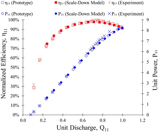
Comparison of performance curves of Francis hydro turbine between experiment and steady CFD analysis[40]
4.2 Internal flow behavior in scale-down mode and prototype
Figure 5 illustrates the vortex rope in the runner passage under partial-load and overload conditions by unsteady CFD analysis. The pressure coefficient (Cp) is used to normalize the pressure magnitude for comparison and is defined using Eq. (10).[12]
| (10) |
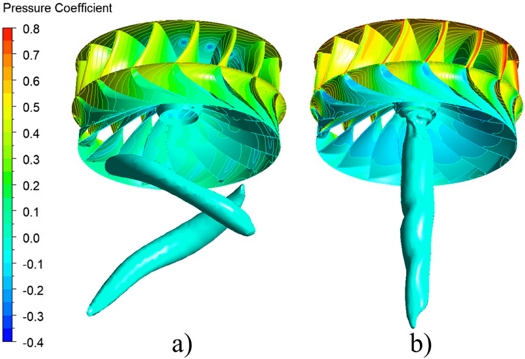
Comparison of vortex rope in the runner flow passage at t=0.94 sec and a) Q11=0.38 and b) Q11=1.00 in scale-down Francis runner model
At Q11=0.38, the flow leaving the runner becomes highly asymmetric, forming an unstable twin vortex rope that induces strong low‑pressure regions throughout the runner flow passage. The pressure coefficient shows a large region of low pressure and intermittent high-pressure patches along the blade surfaces, indicating strong flow asymmetry and swirl flow. At Q11=1.00, the vortex rope becomes shorter, vertical, and stable, indicating more uniform flow attachment and reduced swirl intensity. The vortex rope is more concentrated and axis-aligned, which weakens the draft tube swirl flow. The pressure coefficient is relatively higher at the leading edge than that of Q11=0.38.
Figure 6 illustrates the variation in pressure coefficient (Cp) by unsteady CFD analysis along the normalized blade chord from leading edge (LE) to trailing edge (TE) for both the scale-down and full-scale prototype models at a unit discharge of Q11=0.38. The pressure coefficient magnitudes at the pressure and suction sides are relatively higher in the scale-down model than in the prototype model. At normalized distances 0.6 to 1.0, the crossover of Cp value between the pressure and suction sides for both the scale-down model and prototype, which reduces the output power and induces secondary flow, vortices, and eddies. The differences in pressure coefficient distribution between the scale-down model and prototype are visible in Fig. 6. The greater pressure variation across the blade surface, which leads to increased hydrodynamic excitation and potential structural stress, emphasizes the need for accurate fluid–structure interaction modeling when extrapolating scale-model results to full-scale turbine behavior.
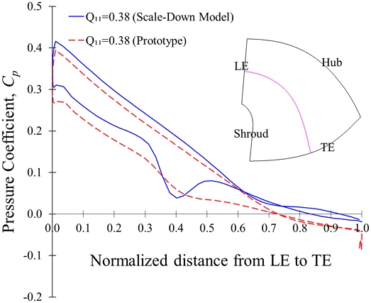
Comparison of pressure coefficient in the runner blade from LE to TE between scale-down and prototype models at Q11=0.38 and t=1.4 sec
Figure 7 presents the pressure coefficient (Cp) distribution for both the scale-down and prototype models at Q11=0.71. The pressure profiles for both configurations show smoother transitions compared to part-load operation, indicating more stable and streamlined flow behavior. However, the prototype still exhibits a slightly higher Cp difference between pressure and suction sides, suggesting slightly stronger fluid acceleration. The close alignment of Cp in the blade surface confirms good geometric similarity and validates the scale model’s predictive capability under optimal operating conditions. Nonetheless, the subtle deviations near the leading and trailing edges highlight the need for careful extrapolation when assessing structural loads and fatigue risks in full-scale turbines.
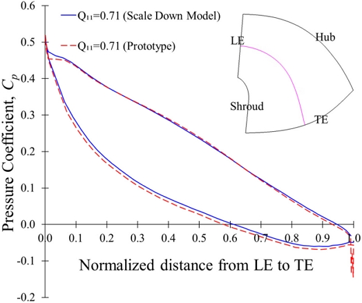
Comparison of pressure coefficient in the runner blade from LE to TE between scale-down and prototype models at Q11=0.71 and t=1.4 sec
Figure 8 illustrates the pressure coefficient using unsteady CFD analysis at a unit discharge of Q11=1.00. At a normalized distance of 0.1, the Cp crossover between the pressure and suction sides is observed. The crossover reduces the output power and the hydraulic efficiency of the scale-down and prototype Francis runner. At the leading edge, pressure on the suction side is relatively higher than on the pressure side. The Cp difference between the suction and pressure sides is relatively higher at Q11=1.00 than at 0.71 and 0.38. The results emphasize the importance of incorporating high-fidelity CFD analysis to accurately assess stress concentrations and fatigue risks in prototype runners operating under a flexible operation range.
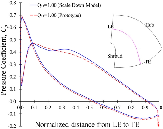
Comparison of pressure coefficient in the runner blade from LE to TE between scale-down and prototype models at Q11=1.00 and t=1.4 sec
Figure 9 compares the Q-criterion by unsteady CFD analysis between the scale-down and prototype models at Q11=0.38. The Q-criterion is a well-known vortex feature definition presented as a non-dimensional quantity with normalized local shear strain rate calculated using Eq. (11).[41] The positive value of the Q-criterion indicates the existence of a vortex region in the flow passage.[42]
| (11) |
| (12) |
| (13) |
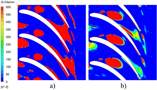
Comparison of Q-criterion by unsteady CFD analysis on the runner blade passages of a) scale-down and b) prototype models at Q11=0.38 and t=1.4sec
The positive value of the Q-criterion is observed at the blade flow passage, which indicates the occurrence of a vortex region in the blade flow passage. The vortex in the blade flow passage influenced the pressure coefficient distribution on the blade surface. At Q11=0.38, the occurrence of a vortex region reduced the pressure difference between the suction and pressure sides. In the scale-down model, the Q-criterion value is significantly higher at the trailing edge, which makes the Cp crossover between the suction and pressure sides of the runner blade. The vortex region location in the blade flow passage is the same, but the magnitude differs between the prototype and the scale-down model. It concludes that the vortex formation patterns are preserved, but their intensity and spatial extent differ due to scale-dependent physics.
4.3 FSI analysis in the Francis turbine for the scale-down and prototype models
The internal flow characteristics and pressure coefficient on the blade surface are obtained using the steady and unsteady CFD analyses. Fig. 10 compares the equivalent stress in the scale-down model with the steady and unsteady CFD analyses at Q11=0.38. The maximum stress of 10 MPa is observed at the blade TE near the hub region. The maximum stress is distributed on the runner shroud region. Fig. 11 shows the total deformation in the scale-down runner domain from the steady and unsteady CFD analysis results at Q11=0.38. The maximum deformation is approximately 0.009 mm and occurred at the shroud region. The stress and deformation contours indicate that the high stress and deformation occurred at the hub and shroud regions of the runner domain, respectively. Fig. 12 compares the stress and deformation in the scale-down model with the steady and unsteady CFD analyses. It indicates that the structural analysis performed using the steady and unsteady analyses matches well. The maximum stress and deformation are observed at Q11=1.00. It concludes that stress and deformation on the runner blade surface gradually increased with increasing flow rates.
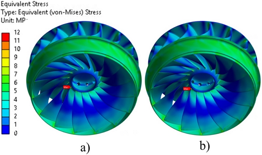
Comparison of equivalent stress with a) steady and b) unsteady CFD analyses at Q11=0.38 in Francis hydro turbine runner scale-down model
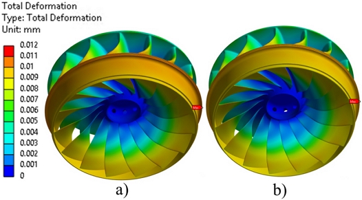
Comparison of total deformation with a) steady and b) unsteady CFD analyses at Q11=0.38 in Francis hydro turbine runner scale-down model
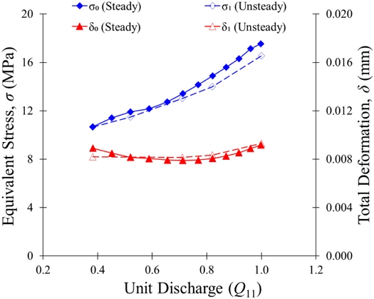
Comparison of equivalent stress and total deformation in the scale-down model according to flow conditions with the steady and unsteady CFD analysis results
Table 5 compares the maximum equivalent stress and total deformation in the scale-down and prototype runners at the flexible operating range. The maximum stresses for the scale-down and prototype models are 117.41 MPa and 16.55 MPa, respectively. Similarly, the maximum total deformations for the scale-down and prototype models are 0.0093 mm and 0.50 mm, respectively. When Q11 increased from 0.38 to 1.00, the maximum equivalent stress and deformation increased by 55% and 13%, respectively, for the scale-down model. Similarly, for the prototype runner, the maximum stress and deformation increased by 13% and 14%, respectively.
Comparison of maximum equivalent stress and total deformation in the scale-down and prototype runners at the flexible operating range
Figure 13 summarizes the variation of equivalent stress and total deformation for the scale‑down and prototype models across the examined unit discharges from unsteady FSI analysis results. The prototype consistently shows higher stresses, approximately 100―120 MPa, across all operating points, whereas the scale‑down model maintains significantly lower levels below 20 MPa, reflecting scale‑related structural stiffness differences and increased hydrodynamic load intensity at full scale. Similarly, the total deformation in the prototype increases from 0.44 mm to 0.50 mm, whereas the scale‑down model shows only minor increases of about 0.008 mm to 0.009 mm, with an increase in Q11 from 0.38 to 1.00, respectively . Both runners exhibit increasing stress and deformation with discharge, but the prototype shows a much steeper trend. These results confirm that scale effects heavily influence structural behavior, demonstrating that scale-down model FSI results cannot be directly extrapolated to full scale without applying appropriate correction or similarity adjustments.
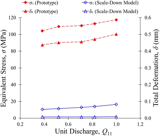
Comparison of equivalent stress and total deformation in the scale-down and prototype runner according to flow conditions with unsteady FSI analysis results
Figures 14 and 15 present the normalized equivalent stress σ11 and normalized total deformation δ11 for both the scale‑down and prototype runner models, respectively, which are calculated using Eqs. (14) and (15). The normalized equivalent stress trends presented in Fig. 14 further clarify how fluid–structure interaction behavior differs between the scale‑down model and the prototype across the flexible operating range.
| (14) |
| (15) |
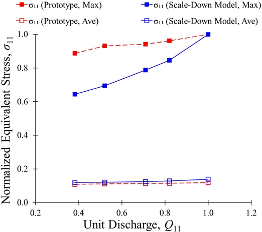
Comparison of normalized equivalent stress in the scale-down and prototype runners according to discharge conditions
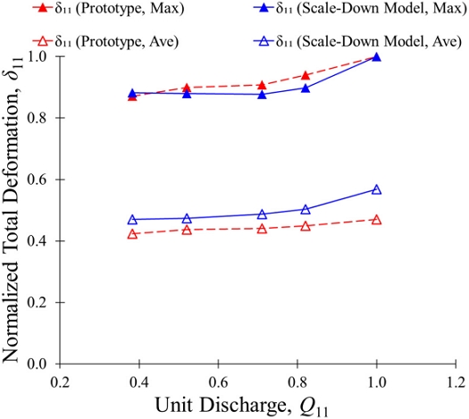
Comparison of normalized total deformation in the scale-down and prototype runners according to discharge conditions
The prototype runner exhibits consistently higher normalized maximum stress values, increasing from approximately Q11=0.38 to Q11=1.00. The scale-down and prototype runner models showed consistently low average normalized stress ranges from 0.10 to 0.15. At Q11=0.38, the normalized maximum stress values are 0.64 and 0.89 for the scale-down and prototype runner models, respectively, in the localized region near the hub and trailing edge. The normalized total deformation trends shown in Fig. 15 highlight distinct structural responses of the scale‑down and prototype runner models across the unit discharges. For both runners, the average normalized deformation remains substantially less than the maximum value, indicating that localized regions near the shroud primarily govern the peak deformation. These trends are consistent with the absolute deformation results, and the prototype undergoes significantly larger physical displacement than the scale‑down model. The gradual increase in normalized average deformation with discharge in both cases confirms that the structural response changes with the flow conditions, while the difference in magnitude underscores the influence of scale effects on the structural behavior of the Francis hydro turbine.
5. Conclusions
The comparative FSI investigation of the scale‑down and prototype Francis turbine runners is demonstrated in this study. The pressure coefficient distributions show that the part‑load operation (Q11=0.38) produces the highest degree of flow non‑uniformity, characterized by sudden decrease in pressure difference near the trailing edge between suction and pressure sides in both runner models. As the flow approaches Q11=0.71 and 1.00, these discrepancies diminish substantially, indicating improved model–prototype similarity under stable hydraulic conditions. The internal flow patterns at higher discharge levels reveal smoother loading, reduced incidence effects at the leading edge, and consistent pressure recovery across the blade span.
The structural results further emphasize the influence of scaling on runner behavior. The magnitude of stress and deformation differs between the scale-down and prototype models. While the scale‑down model exhibits relatively low stress levels (<20 MPa) and very small deformations (<0.01 mm), the full‑scale runner experiences substantially higher stresses (100―120 MPa) and absolute deformations (0.44―0.50 mm) across the flexible operating range. When Q11 increases from 0.38 to 1.00, the equivalent stress and deformation increase by 55% and 13% for the scale-down models, and by 13% and 14% for the prototype Francis hydro turbine models, respectively. The results show that CFD analysis successfully captured the overall hydraulic trends of both the scale‑down and prototype models, particularly at the BEP. However, directly extrapolating stresses or deformations from the scale‑down model to the prototype can be misleading, especially under part‑load conditions where flow instabilities dominate.
In future work, modal analysis will be performed to investigate resonance risks associated with hydraulic excitation frequencies.
Nomenclature
| [C] : | damping matrix |
| [K] : | stiffness matrix |
| [M] : | mass matrix |
| {F} : | nodal load vector |
| {a} : | acceleration |
| {v} : | velocity |
| {x} : | displacement |
| Bx : | strain-displacement matrix |
| Cp : | pressure coefficient |
| D : | reference diameter, m |
| Dp : | reference diameter of prototype, m |
| Dm : | reference diameter of scale-down model, m |
| E : | specific hydraulic energy, J/kg |
| Es : | structural elasticity matrix of francis turbine |
| G : | grid number |
| g : | acceleration due to gravity, m/s2 |
| H : | head, m |
| N : | rotational speed, min-1 |
| Ns : | specific speed |
| N11 : | unit speed |
| P : | output power, kW |
| P11 : | unit power, kW |
| p : | pressure, kPa |
| pref : | reference pressure at draft tube outlet, kPa |
| Q : | flow rate, m3/s |
| Q11 : | unit discharge |
| Qc : | q-criterion, s-1 |
| r : | grid refinement factor |
| S : | rate of strain tensor |
| ▽u : | velocity gradient tensor |
| [▽u ]T : | transpose of velocity gradient tensor |
| Ω : | rotation (vorticity) tensor |
| α : | mass-proportional damping coefficient |
| β : | stiffness-proportional damping coefficient |
| εa : | approximate relative error |
| εext : | extrapolated relative error |
| δ : | total deformation, mm |
| δ0 : | total deformation by steady FSI analysis, mm |
| δ1 : | total deformation by unsteady FSI analysis, mm |
| δm : | maximum total deformation at Q11=1.00, mm |
| δ11 : | normalized total deformation |
| η11 : | normalized efficiency |
| ηBEP@Exp. : | efficiency at BEP from experimental analysis |
| ρ : | density of water at 25°C, 997 kg/m3 |
| σ : | equivalent stress, MPa |
| σ0 : | equivalent stress by steady FSI analysis, MPa |
| σ1 : | equivalent stress by unsteady FSI analysis, MPa |
| σf : | flow induced stress, MPa |
| σm : | maximum equivalent stress at Q11=1.00, MPa |
| σ11 : | normalized equivalent stress |
| σmax : | maximum principal stress, MPa |
| σmid : | middle principal stress, MPa |
| σmin : | minimum principal stress, MPa |
Acknowledgments
This work is supported by KOREA HYDRO & NUCLEAR POWER CO, LTD (No. H24S046000).
References
- International Energy Agency, 2021, “Hydropower special market report: Analysis and forecast to 2030”, OECD Publishing, https://iea.blob.core.windows.net/assets/4d2d4365-08c6-4171-9ea2-8549fabd1c8d/HydropowerSpecialMarketReport_corr.pdf, .
-
Karekezi, Y.C., Maurer, F., Robles, D.J.T., Oyvang, T., and Noland, J.K., 2025, “Transforming Classical Hydropower Generation for Flexibility in the Global Energy Transition: Challenges, Requirements, and Prospects”, IEEE Access, 13, 74762-74780.
[https://doi.org/10.1109/ACCESS.2025.3564123]

-
Goyal, R., and Gandhi, B.K., 2018, “Review of hydrodynamics instabilities in Francis turbine during off-design and transient operations”, Renew. Energy, 116, 697-709.
[https://doi.org/10.1016/j.renene.2017.10.012]
-
Trivedi, C., and Cervantes, M.J., 2017, “Fluid-structure interactions in Francis turbines: A perspective review”, Renew. Sustain. Energy Rev., 68, 87-101.
[https://doi.org/10.1016/j.rser.2016.09.121]
- Alligne, S., Nicolet, C., Allenbach, P., Kawkabani, B., Simond, J.J., and Avellan, F., 2008, “Influence of the vortex rope location of a Francis turbine on the hydraulic system stability”, Proc. 24th Symposium on Hydraulic Machinery and Systems, 1-10, https://www.hdynamics.ch/Profile/Publications/pdf/IAHR_2008_82.pdf, .
-
Ciocan, G.D., Iliescu, M.S., Vu, T.C., Nennemann, B., and Avellan, F., 2007, “Experimental Study and Numerical Simulation of the FLINDT Draft Tube Rotating Vortex”, J. Fluids Eng., 129(2), 146-158.
[https://doi.org/10.1115/1.2409332]
-
Ni, Y., Zhu, R., Zhang, X., and Pan, Z., 2018, “Numerical investigation on radial impeller induced vortex rope in draft tube under partial load conditions”, J. Mech. Sci. Technol., 32(1), 157-165.
[https://doi.org/10.1007/s12206-017-1217-7]
-
Ji, L., Xu, L., Peng, Y., Zhao, X., Li, Z., Tang, W., and Liu, X., 2022, “Experimental and numerical simulation study on the flow characteristics of the draft tube in Francis turbine”, Machines, 10(4), 230.
[https://doi.org/10.3390/machines10040230]
-
Trivedi, C., and Dahlhaug, O.G., 2018, “Interaction between trailing edge wake and vortex rings in a Francis turbine at runaway condition: Compressible large eddy simulation”, Physics of Fluids, 30(7), 075101.
[https://doi.org/10.1063/1.5030867]
-
Valentín, D., Presas, A., Egusquiza, E., Valero, C., Egusquiza, M., and Bossio, M., 2017, “Power swing generated in Francis turbines by part load and overload instabilities”, Energies, 10(12), 2124.
[https://doi.org/10.3390/en10122124]
-
Zanetti, G., Cavazzini, G., and Santolin, A., 2023, “Effect of the von Karman shedding frequency on the hydrodynamics of a Francis turbine operating at nominal load”, Int. J. Turbomach. Propuls. Power, 8(3), 27.
[https://doi.org/10.3390/ijtpp8030027]
- International Electrotechnical Commission, 1999, “IEC 60193: Hydraulic turbines, storage pumps and pump-turbines—model acceptance tests”.
- International Electrotechnical Commission, 1991, “IEC 60041: Field acceptance tests to determine the hydraulic performance of hydraulic turbines. Storage, pumps and pump turbines”.
-
Wu, Y., Liu, S., Dou, H.S., Wu, S. and Chen, T., 2012, “Numerical prediction and similarity study of pressure fluctuation in a prototype Kaplan turbine and the model turbine”, Computers & Fluids, 56, 128-142.
[https://doi.org/10.1016/j.compfluid.2011.12.005]
-
Gülich, J. F., 2010, “Operation of centrifugal pumps. In Centrifugal pumps”, In: Centrifugal Pumps. Springer, Berlin, Heidelberg.
[https://doi.org/10.1007/978-3-642-12824-0_11]
- Avellan, F., 2004, “Introduction to cavitation in hydraulic machinery”, Proc. 6th International Conference on Hydraulic Machinery and Hydrodynamics, Timisoara, Romania, 11-22.
-
Menter, F.R., 1994, “Two-equation eddy-viscosity turbulence models for engineering applications”, AIAA J., 32(8), 1598-1605.
[https://doi.org/10.2514/3.12149]
-
Sahu, P., Subbarao, P.M.V., and Goyal, R., 2026, “High-fidelity simulations and validations of Francis turbine: a comprehensive review on conventional and modern modelling techniques”, J. Braz. Soc. Mech. Sci. Eng., 48, 68.
[https://doi.org/10.1007/s40430-025-06019-5]
-
Wang, W. Q., Zhang, L. X., Yan, Y., and Guo, Y., 2007, “Large-eddy simulation of turbulent flow considering inflow wakes in a Francis turbine blade passage”, J. Hydrodyn., 19(2), 201-209.
[https://doi.org/10.1016/S1001-6058(07)60049-3]
-
Jošt, D., and Lipej, A., 2011, “Numerical prediction of non-cavitating and cavitating vortex rope in a Francis turbine draft tube”, Stroj. Vestn.-J. Mech. Eng., 57(6), 445-456.
[https://doi.org/10.5545/sv-jme.2010.068]
-
Celik, I.B., Ghia, U., Roache, P.J., and Freitas, C.J., 2008, “Procedure for estimation and reporting of uncertainty due to discretization in CFD applications”, J. Fluids Eng., 130(7), 078001.
[https://doi.org/10.1115/1.2960953]
-
Pope, S.B., 2000, “Turbulent flows”, Meas. Sci. Technol., 12(11), 2020-2021.
[https://doi.org/10.1088/0957-0233/12/11/705]
-
Dettmer, W.G., and Perić, D., 2013, “A new staggered scheme for fluid–structure interaction”, Int. J. Numer. Methods Eng., 93(1), 1-22.
[https://doi.org/10.1002/nme.4370]
-
Kan, K., Zheng, Y., Zhang, X., Yang, C., and Zhang, Y., 2015, “Numerical study on unidirectional fluid–solid coupling of Francis turbine runner”, Adv. Mech. Eng., 7(3).
[https://doi.org/10.1177/1687814015568938]
-
Escaler, X., Egusquiza, E., Farhat, M., Avellan, F., and Coussirat, M., 2006, “Detection of cavitation in hydraulic turbines”, Mech. Syst. Signal Process., 20(4), 983-1007.
[https://doi.org/10.1016/j.ymssp.2004.08.006]
-
Elhami, M.R., Najafi, M.R., and Tashakori Bafghi, M., 2021, “Vibration analysis and numerical simulation of fluid–structure interaction phenomenon on a turbine blade”, J. Braz. Soc. Mech. Sci. Eng., 43(5), 245.
[https://doi.org/10.1007/s40430-021-02933-6]
-
Unterluggauer, J., Doujak, E., and Bauer, C., 2019, “Numerical fatigue analysis of a prototype Francis turbine runner in low-load operation”, Int. J. Turbomach. Propuls. Power, 4(3), 21.
[https://doi.org/10.3390/ijtpp4030021]
-
Bendat, J.S., and Piersol, A.G., 2011, “Random data: analysis and measurement procedures”, 4th ed., John Wiley & Sons, Hoboken.
[https://doi.org/10.1002/9781118032428]
-
Welch, P.D., 1967, “The use of fast Fourier transform for the estimation of power spectra: A method based on time averaging over short, modified periodograms”, IEEE Transactions on Audio and Electroacoustics, 15(2), 70-73.
[https://doi.org/10.1109/TAU.1967.1161901]
-
Harris, F.J., 1978, “On the use of windows for harmonic analysis with the discrete Fourier transform”, Proc. IEEE, 66(1), 51-83.
[https://doi.org/10.1109/PROC.1978.10837]
- ASME, 2011, “PTC 18–2011: Hydraulic turbines and pump‑turbines performance test code”, American Society of Mechanical Engineers.
- International Organization for Standardization (ISO), 2012, “ISO 9906:2012 Rotodynamic pumps — Hydraulic performance acceptance tests-Grades 1, 2 and 3”, ISO, https://www.iso.org/standard/41202.html, .
- Ewins, D.J., 2009, “Modal testing: theory, practice and application”, 2nd ed., John Wiley & Sons.
-
Pierre, C., and Dowell, E.H., 1987, “Localization of vibrations by structural irregularity”, J. Sound Vib., 114(3), 549-564.
[https://doi.org/10.1016/S0022-460X(87)80023-8]
- Rao, J.S., 1991, “Turbomachine blade vibration”, New Age International.
-
Franc, J.P. and Michel, J.M., 2005, “Fundamentals of cavitation”, Dordrecht: Springer Netherlands.
[https://doi.org/10.1007/1-4020-2233-6]
-
Arndt, R.E., Voigt Jr, R.L., Sinclair, J.P., Rodrique, P., and Ferreira, A., 1989, “Cavitation erosion in hydroturbines”, J. Hydraul. Eng., 115(10), 1297-1315.
[https://doi.org/10.1061/(ASCE)0733-9429(1989)115:10(1297)]
-
Li, X., Cao, J., Zhuang, J., Wu, T., Zheng, H., Wang, Y., Zheng, W., Lin, G., and Wang, Z., 2022, “Effect of Operating Head on Dynamic Behavior of a Pump–Turbine Runner in Turbine Mode”, Energies, 15(11), 4004.
[https://doi.org/10.3390/en15114004]
-
Liu, X., Huang, X., Chen, W., and Wang, Z., 2025, “Flow-induced strength analysis of large Francis turbine under extended load range”, Appl. Sci., 15(5), 2422.
[https://doi.org/10.3390/app15052422]
- KHNP, 2023, “Model Acceptance Test Report”, Korea Hydro and Nuclear Power.
-
Fu, J., Yuan, Y., and Vigevano, L., 2022, “Numerical investigations of the vortex feature-based vorticity confinement models for the assessment in three-dimensional vortex-dominated flows”, Meccanica, 57(7), 1657-1676.
[https://doi.org/10.1007/s11012-022-01525-5]
- Hunt, J.C., Wray, A.A. and Moin, P., 1988, “Eddies, streams, and convergence zones in turbulent flows”, Studying turbulence using numerical simulation databases, 2. Proc. 1988 summer program, 193-208, https://ntrs.nasa.gov/api/citations/19890015184/downloads/19890015184.pdf, .