
Online publication date 24 Aug 2026
Quantitative Evaluation of Cavitation-Instability Parameters in Francis Hydro Turbine

Copyright © 2026 by the New & Renewable Energy
This is an Open Access article distributed under the terms of the Creative Commons Attribution Non-Commercial License (http://creativecommons.org/licenses/by-nc/4.0) which permits unrestricted non-commercial use, distribution, and reproduction in any medium, provided the original work is properly cited.
Abstract
This paper presents a quantitative evaluation of cavitation-induced instabilities in a Francis hydroturbine. This approach combines a one-dimensional (1D) hydroacoustic model with three-dimensional (3D) CFD analysis. The 1D model incorporates hydraulic inductance, resistance, and draft-tube geometric divergence, as well as cavitation parameters such as wave speed, cavitation compliance, mass-flow gain factor, and bulk viscosity. This enables the prediction of pressure fluctuations, draft-tube cavitation behavior, and transient shutdown characteristics. Complementary 3D CFD simulations using ANSYS CFX yield detailed performance curves of the turbine. The 1D model captures the dynamic hydraulic behavior during guide-vane closure. The combined approach identifies unstable operating regions and characterizes the cavitation compliance, mass-flow gain factor, and wave-speed variation as functions of discharge and cavitation number. It provides a robust framework for evaluating dynamic mechanisms governing cavitation instability in Francis turbines.
Keywords:
Francis hydro turbine, Cavitation, Numerical analysis, Cavitation compliance, Mass flow gain factor, Wave speed키워드:
프란시스 수차, 캐비테이션, 수치 해석, 캐비테이션 순응도, 질량유량 증가계수, 파동속도1. Introduction
The vortex rope dynamics in Francis hydro turbines constitute a critical hydrodynamic instability that directly influences turbine performance and structural reliability.[1~3] Under off-design operation, the swirling flow at the runner outlet evolves into a helical or axisymmetric vortex rope in the draft tube, producing pressure pulsations and vibrations that can reduce turbine lifespan.[1,3] To analyze such behavior, researchers employ both one‑dimensional (1D) and three‑dimensional (3D) computational analysis approaches, where 1D hydroacoustic models such as SIMSEN offer rapid prediction of pressure‑wave propagation and system‑level instabilities[1] while 3D CFD simulations provide high‑fidelity characterization of vortex structures, turbulence physics, and cavitation development.[4,5]
As modern hydropower plants increasingly operate under flexible, variable‑load conditions, Francis turbines spend more time away from the best efficiency point (BEP), where part‑load swirl promotes the formation of a precessing vortex rope (typically 0.2–0.4 fn).[3,6] At full load, stronger cavitation and high discharge can trigger an axisymmetric surge, a more severe oscillatory mode.[2,7] These pressure instabilities can couple with the hydraulic system, leading to resonance, power swings, and significant mechanical loading.[8] Prior investigations have shown that cavitation compliance, mass flow gain factor, and bulk viscosity are fundamental parameters governing rope development and hydroacoustic feedback.[9] Additional findings from laboratory measurements and high-resolution CFD have revealed deep partial load pulsations, lock-in behavior, and complex interactions between the swirling flow and draft tube geometry.[10,11] Despite extensive research, a need remains for fast and reliable prediction tools to evaluate instability regions during design and real-time operation.[12] SIMSEN enables hydroacoustic eigenvalue analysis, unsteady transient simulation, and integrated modeling of turbine–waterway interactions[7], while CFD methods based on RANS and turbulence modeling accurately capture swirling, separation, and cavitation structures in the draft tube.
Therefore, this study aims to demonstrate that by combining 1D and 3D modeling strategies, engineers can achieve a robust, multiscale understanding of vortex‑rope dynamics and develop more stable and efficient Francis turbine systems.
2. Modeling and Methodology
2.1 Francis Hydro Turbine Modeling
The specific speed of the Francis hydro turbine is 147 [min-1, kW, m]. Francis hydro turbine is designed accordingly. Fig. 1 shows the 3D modeling of the Francis hydro turbine model. The CAD view shows the spiral casing, stay–guide cascade, runner, and draft tube. The design specifications of the Francis hydro turbine are shown in Table 1, which are calculated using Eqs (1)-(4).
| (1) |
| (2) |
| (3) |
| (4) |
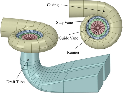
3D modeling of Francis hydro turbine

Specification of Francis hydro turbine model
2.2 1D Analysis of Francis Hydro Turbine
SIMSEN is used for the 1D analysis. The continuity and momentum equations are solved by neglecting the convective terms and assuming a plane pressure wave and a uniform field in a cross-section. The hyperbolic partial differential equations are solved by the finite difference method, employing a first‑order centered scheme discretization.
Fig. 2 represents a 1D model of a cavitation-free pipe. The continuity and momentum conservation equations for a cavitation-free pipe are described in Eq. (5), and their electrical analogy is described in Eq. (6), where L', R', and C' are lineic impedance, lineic resistance, and lineic capacitance values.[13] The given pipe is simulated as a combination of elements with a constant length of dx. For each element, the hydraulic impedance L, resistance R, and capacitance C are then defined as L =L'dx, R =R'dx, and C =C'dx, respectively. The resulting electrical analogy of a cavitation-free pipe is shown in Fig. 2b). Fig. 3 shows the Francis hydro turbine model and its electrical analogy circuit. The dynamic behavior of the Francis hydro turbine model is evaluated using the guide vane closure effect (Rt), water inertia (Lt), and energy transfer in the runner flow passage (Ht). The turbine is described along the hydraulic grade line, showing how the upstream total head (H1), downstream tailwater head (H2), and inlet pressure head define the net available head driving the flow (Q), while runner rotation (ω) and guide‑vane opening determine the turbine’s characteristic curves. The resulting equivalent model of the Francis turbine runner is described by an inductance, resistance, and pressure source, which is given by Eq. (7). The electrical equivalent of the 1D SIMSEN hydro-acoustic model of a cavitating draft tube cone is illustrated in Fig. 4. The cavitation model developed by Alligne et al.,[1] in which dissipation due to the velocity gradient induced by the compressibility of the cavitation volume is taken into account. The hydraulic inductance (L) and resistance (Rλ') are used to evaluate fluid inertia and energy losses, respectively. The occurrence of cavitation volumes in the draft tube decreases the wave speed, which is described by the parameter J'. The destabilizing effect of the divergent geometry of the draft tube is modeled using Rd'. The resistance Rμ' is used to evaluate the thermodynamic equilibrium between the cavitation volume and the surrounding liquid. The continuity and momentum equations for cavitation flow in the draft tube are shown in Eq. (8). Fig. 5 shows a basic 1D Francis hydro turbine model, comprising the upper reservoir, penstock pipe, Francis turbine model, and lower reservoir.
| (5) |
| (6) |
| (7) |
| (8) |
| (9) |
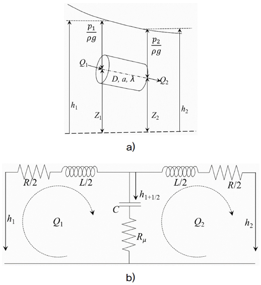
1D pipe model without cavitation a) hydraulic model and b) equivalent electrical circuit[9]
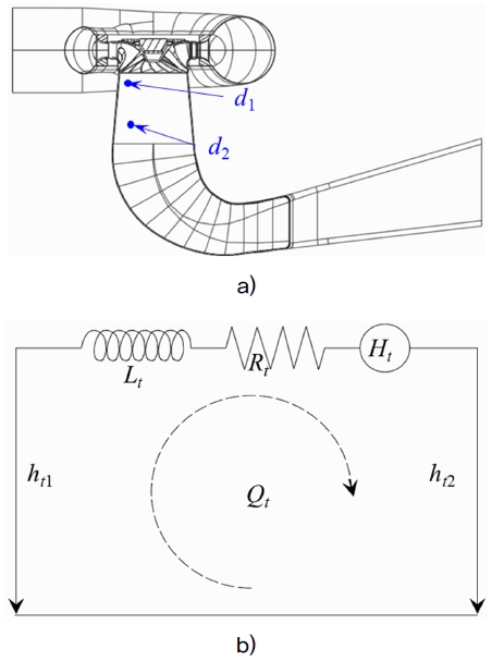
1D Francis hydro turbine model a) hydraulic model and b) equivalent electrical circuit[9]
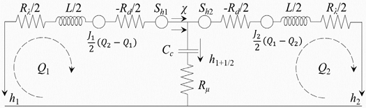
Representation of 1D model of cavitation vortex rope in the draft tube[9]
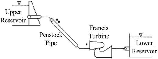
Basic 1D model of Francis hydro turbine model using SIMSEN[9]
2.3 Numerical Methodology of 3D CFD Analysis
It is possible to determine the required parameters directly from CFD simulations. In this approach, single‑phase incompressible flow analysis is performed. Furthermore, a homogeneous mixture of water and water vapor is used for the cavitation analysis; the corresponding water vapor volume fraction can be extracted from the CFD analysis. This procedure enables a consistent evaluation of cavitation‑induced flow in the Francis hydro turbine model. ANSYS 2024R2 is used to conduct 3D CFD analysis of the Francis hydro turbine.[14] The computational domain of the Francis hydro turbine consists of the spiral casing, stay vanes, guide vanes, runner, and draft tube, as shown in Fig. 1. A hexahedral dominant grid topology was generated using ANSYS ICEM 2024R2, providing high accuracy in capturing boundary‑layer gradients and maintaining low numerical dissipation in regions with strong streamline curvature. Fig. 6 shows the numerical grids for each component of the Francis hydro turbine. Fig. 7 shows the mesh dependency test for the optimum mesh number selection, which is 9.26 million nodes with max. y+ value is 30 for the runner flow passage. The full domain was utilized for the 3D CFD analysis. Reynolds-Averaged Navier–Stokes (RANS) equations were solved with the finite‑volume solver ANSYS CFX 2024R2. For steady‑state simulations, the Shear Stress Transport (SST) turbulence model was selected for steady analysis, respectively, because of its effectiveness in resolving adverse pressure gradients along blade surfaces.[15] At the inlet, a total pressure boundary condition was applied, while static pressure was specified at the outlet. All wall boundaries were treated as no‑slip, with automatic wall functions employed. The detailed steady and unsteady 3D CFD analysis method for the Francis hydro turbine applied in this study can be found in the related research results.[16,17] Table 2 shows the 3D CFD analysis specifications for the Francis hydro turbine model.
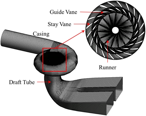
Numerical grids for Francis hydro turbine components for the CFD analysis
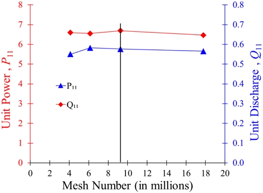
Grid dependency test for 3D CFD analysis
Specification for 3D CFD analysis of Francis turbine model
3. Results and Discussion
3.1 Performance Curves of the Francis Hydro Turbine Model
The unit efficiency (η11) is used to evaluate the performance of the experiment and 3D CFD analysis. Fig. 8 compares η11 and P11 against Q11 for both experiment and 3D CFD analysis of the Francis turbine models.
| (10) |
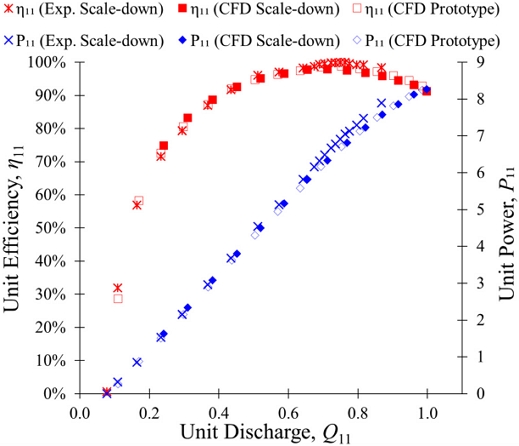
Performance curves comparison between experiment and 3D CFD analysis of Francis hydro turbine model[18]
The η11 by experiment for the scale-down model increases rapidly, reaching a peak value, after which it slightly decreases. The same tendency is observed for scale-down and prototype models with CFD analysis. The P11 increases linearly with Q11, reaching approximately 8.2–8.5 at full load conditions. Overall, the CFD results match the experimental curves well, confirming the accurate prediction of turbine performance. The relative errors between experimental and 3D CFD analysis for η11 and P11 are less than 2.0% and 4.0% throughout the operating range. The small discrepancies demonstrate that the 3D CFD analysis reproduces the experimental trends with high fidelity, validating the reliability of the CFD approach.
3.2 Efficiency Hill Chart of the Francis Hydro Turbine Model
Fig. 9 presents the efficiency hill chart of the Francis turbine model by 3D CFD analysis, showing η11 contours superimposed on the Q11–η11 operating plane together with guide vane opening lines. The highest efficiency is centered around η11≈0.99, occurring at η11≈62 and Q11≈0.71, corresponding to the best efficiency point (BEP). The surrounding efficiency contours decrease gradually to 0.98, 0.97, 0.96, and so on, forming closed elliptical shapes that indicate stable and smooth hydraulic performance. At Q11<0.6 and η11>65, the efficiency drops below 0.92 due to incidence losses. At Q11<0.6, the flow angle entering the runner blades deviates significantly from the designed blade angle. At η11>65, the relative velocity at the blade inlet increases, amplifying the incidence effect and intensifying flow separation. The combination of low discharge and high speed reduces the turbine efficiency. The efficiency hill chart identifies the optimal speed-discharge combinations for maximum turbine performance.
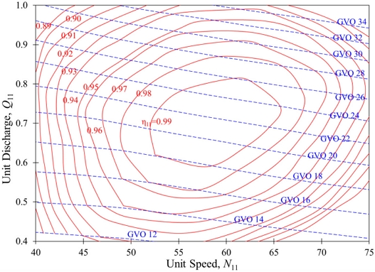
Efficiency hill chart of Francis hydro turbine model by 3D CFD Analysis
3.3 1D Analysis of Francis Hydro Turbine
The pressure coefficient (Cp) is used to normalize the pressure fluctuation and is calculated using Eq. (11).
| (11) |
Fig. 10 compares the pressure coefficient fluctuations at the draft tube inlet (d1) and outlet (d2) at Q11=0.71, and the measurement points are indicated in Fig. 3a). For the 3D CFD simulations, the dominant unsteady phenomena are associated with runner rotation and RSI. The analysis of the pressure time histories shows that after an initial transient period of approximately 1.0–1.5 sec, the signal reaches a statistically stationary oscillatory state. The 1D SIMSEN model, which has significantly lower computational cost, was simulated for 10 sec to assess long-term hydroacoustic behavior. Although different simulation durations are used, the comparison in Fig. 10 is performed using the converged portions of the respective responses. The Cp at the inlet and outlet of the draft tube shows the same tendency between 1D and 3D CFD analyses. The 3D CFD analysis was performed for 2 sec due to the relatively high computational cost compared to the 1D analysis results. The average Cp value is consistent with both analyses, and the results match well over time. At the draft tube inlet and outlet, pressure fluctuations with high and low frequencies are observed, which are related to turbulent shear layer activity near the runner outlet and cavitation vortex rope oscillation, respectively.
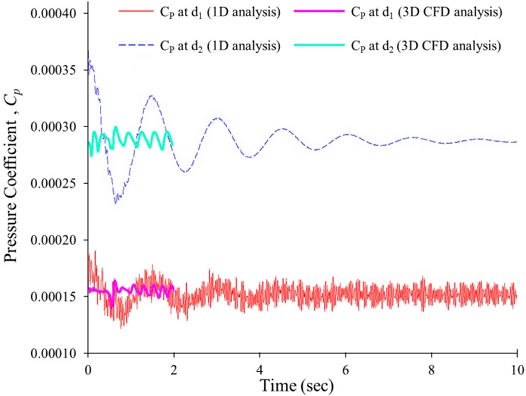
Comparison of Cp fluctuation in the draft tube during cavitation by 1D and 3D CFD analyses at Q11=0.71
Fig. 11 shows the transient variation of Cp at the draft tube inlet together with the unit discharge Q11 during turbine shutdown. As the guide vanes begin closing at around 10 sec, the unit discharge decreases from 0.70 to 0.45 by 12 sec, further decreases to 0.20 by 15 sec. Correspondingly, Cp drops sharply from 0.0 to approximately –0.25, indicating a severe pressure depression in the draft tube caused by rapid flow deceleration and increased swirl intensity. Between 10 sec and 20 sec, the pressure exhibits large amplitude oscillations as the flow passes through unstable part‑load conditions. The trend highlights a gradual increase in flow separation and vortex strength in the runner flow passage during shutdown, which deteriorates the flow in the draft tube flow passage.[19,20] Fig. 11 shows the strong coupling between flow reduction and draft tube pressure fluctuations during a transient shutdown.
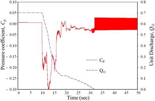
Pressure coefficient fluctuation in draft tube at d1 with decrease in flow rate by 1D analysis
The dynamic behavior illustrated in Fig. 12 highlights the ability of the 1D model to capture transient phenomena of a Francis turbine during shutdown, showing the time‑dependent evolution of head (H), flow rate (Q), and torque (T) expressed in per‑unit values. This simulation represents a typical guide vane closing, forcing the turbine to transition from steady operation to complete stoppage. The curves capture the inherent hydraulic inertia and unsteady load exchanges that occur during rapid changes in operating conditions. At the beginning of the transient analysis, the turbine operates steadily with constant values of normalized head, discharge, and torque. The flow remains fully aligned with the runner blades, and no significant fluctuations are observed. Once the shutdown maneuver begins at around 10 sec, the guide vanes start to close, triggering an immediate reduction in discharge.
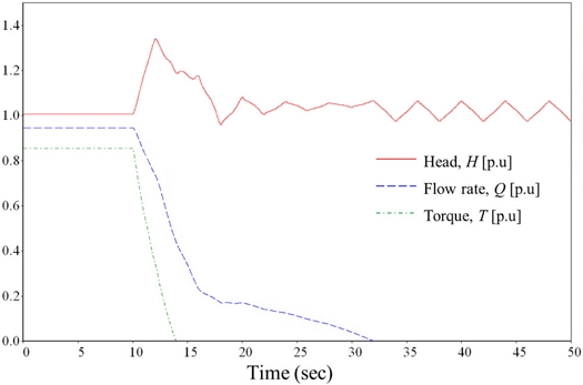
Dynamic behavior of the Francis hydro turbine with closing guide vane opening by ID analysis
3.4 FFT Analysis of Unsteady Flow in the Francis Hydro Turbine Model
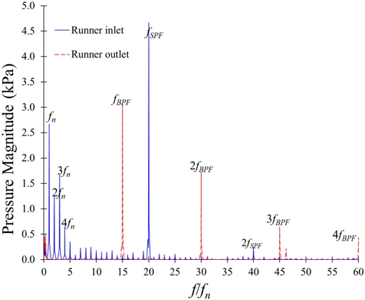
Fig. 13 illustrates the pressure coefficient distribution in the Francis turbine runner and draft tube obtained from 3D CFD analysis. The high-pressure regions are connected at the runner inlet, while low-pressure zones and swirling structures develop toward the runner outlet and draft tube. The helical vortex rope is observed in the draft tube of a Francis hydro turbine. The Fast Fourier Transform (FFT) analysis elaborates on the occurrence of vortex structure in the Francis hydro turbine. The runner rotational frequency, blade passing frequency, and stator passing frequency are explained in Eq. (12).
| (12) |
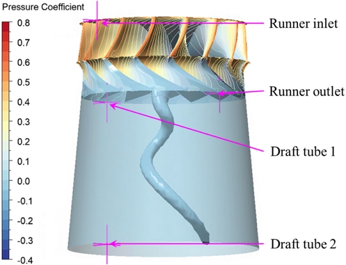
Vortex rope visualization in Francis hydro turbine draft tube at Q11=0.71 with measuring points
Fig. 14 shows the pressure fluctuation at the runner inlet and outlet. At the runner inlet, the dominant peak of 4.67 kPa at fSPF confirms strong RSI caused by periodic interaction between rotating runner blades and stator induced wakes. Additionally, several peaks appear at the integral multiples of fn, which are associated with inlet flow non-uniformity, swirl flow, and large-scale vortices. At the runner outlet, the sharp peaks of pressure 3.09 kPa, 1.72 kPa, 0.69 kPa, and 0.43 kPa appear at fBPF, 2fBPF, 3fBPF, and 4fBPF, respectively, reflecting RSI and blade wake dynamics.
FFT analysis in runner flow passage at Q11=0.71 by 3D CFD analysis
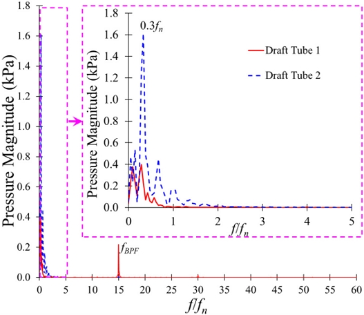
Fig. 15 illustrates the pressure spectrum in the draft tube, which is dominated by low-frequency components. The most prominent pressure peak is 1.6 kPa, which appeared at 0.3fn, while high-frequency components are attenuated in the draft tube flow passage. A low-frequency peak corresponds directly to the precessing motion of the vortex rope visualized in Fig. 13 and represents vortex rope induced pressure pulsations rather than RSI. The strong attenuation of higher frequency components in the draft tube further indicates that RSI effects are largely dissipated downstream. The FFT spectrum analysis demonstrates that RSI dominates the unsteadiness near the runner, whereas vortex rope dynamics control the pressure fluctuations within the draft tube flow passage.
FFT analysis in draft tube flow passage at Q11=0.71 by 3D CFD analysis
3.5 Evaluation of Cavitation Parameters
The cavitation number (σ) is a non-dimensional parameter that quantifies the likelihood of cavitation in the hydro turbine and is defined in Eq. (12). It indicates the possibility of the formation of vapor bubbles in the Francis hydro turbine at various operating conditions.
| (13) |
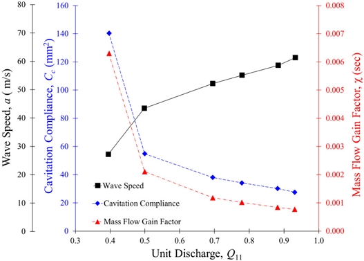
Fig. 16 illustrates the variation of cavitation parameters with unit discharge Q11 at σ=0.033. The cavitation compliance and mass flow gain factor reach their maximum at Q11≈0.35, then decrease sharply up to Q11≈0.50, after which they continue to decline gradually as the discharge increases. In contrast, the wave speed exhibits the opposite trend: starting at a low value for small Q11, it rises with increasing flow rate. This inverse relationship indicates that low‑discharge operating conditions correspond to higher compressibility of the water–vapor mixture, reflected in the large cavitation compliance and mass flow gain factor.
Cavitation parameters variation according to unit discharge at σ=0.033 by ID analysis
The same relationship is reinforced in Fig. 17, which analyzes cavitation parameters as functions of cavitation number σ at Q11=0.71. At σ<0.03, the cavitation compliance and mass flow gain factor remain high and nearly constant, while the wave speed stays close to its minimum value. As the cavitation number increases beyond this region, the compliance decreases sharply and approaches near zero at σ=0.06, indicating a rapid loss of mixture compressibility as cavitation collapses. Correspondingly, the wave speed value is below 60 m/s when the cavitation vortex rope is present in the draft tube[21] and above 1000 m/s in the absence of water vapor volume fraction.[13] Fig. 17 concludes that a cavitation vortex occurs in the Francis hydro turbine model when the cavitation number is less than 0.035. This steep increase in wave speed marks the transition from a vapor‑laden, highly compressible mixture to an almost entirely liquid flow with very high acoustic stiffness.
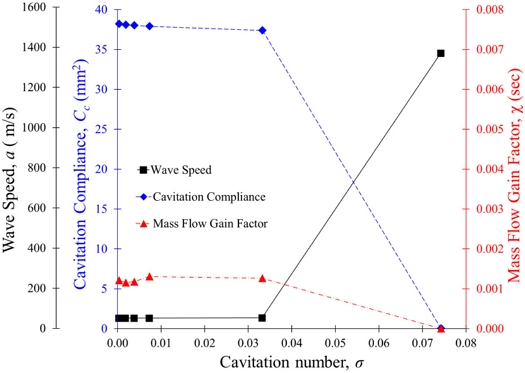
Cavitation parameters variation according to cavitation number at Q11=0.71 by ID analysis
4. Conclusion
A comprehensive numerical assessment of cavitation-related instabilities in a Francis hydro turbine was conducted using 1D SIMSEN hydroacoustic modeling supported by detailed 3D CFD analysis. The 1D model successfully reproduced key transient phenomena, including guide vane closure–driven discharge reduction, rapid torque collapse, draft tube pressure depression, and subsequent damped oscillations resulting from hydraulic inertia. The FFT analysis at the runner and the draft tube flow passage shows high-frequency turbulence-induced fluctuations and RSI near the runner and low‑frequency cavitation volume oscillations associated with the vortex rope. Furthermore, the parametric evaluation of cavitation compliance, mass flow gain factor, and wave speed revealed strong sensitivity to unit discharge and cavitation number, clarifying the conditions under which mixture compressibility dominates acoustic response. Together, the 1D and 3D modeling results provide a reliable and efficient framework for identifying cavitation‑driven instabilities, predicting the draft tube surge behavior, and guiding operational and design strategies aimed at improving the hydraulic stability and performance of the Francis turbines.
Nomenclature
| a : | wave speed |
| A : | cross-section area, m2 |
| B1 : | inlet width of runner, m |
| BEP : | Best Efficiency Point |
| Cc : | cavitation compliance |
| Cp : | pressure coefficient |
| d1 : | draft tube inlet point |
| d2 : | draft tube outlet point |
| D : | reference diameter, m |
| D1 : | inlet diameter of runner, m |
| fn : | runner rotational frequency, Hz |
| fBPE : | blade passing frequency, Hz |
| fSPE : | stator passing frequency, Hz |
| g : | acceleration due to gravity, m/s2 |
| GVO : | Guide Vane Opening |
| H : | effective head, m |
| Ht : | turbine head, m |
| J : | pressure source |
| Jt : | rotational inertia, kg.m2 |
| kx : | cross-section expansion rate |
| L : | hydraulic inductance |
| N : | rotational speed, min-1 |
| N11 : | unit speed |
| Ns : | specific speed |
| pout : | outlet pressure of Francis hydro turbine, Pa |
| pvap : | saturated water vapor pressure at 25°C, Pa |
| P : | shaft power, kW |
| P11 : | unit power |
| Q : | flow rate, m3/s |
| Q11 : | unit discharge |
| RSI : | rotor-stator interaction |
| Rd : | hydraulic divergent resistance |
| Rλ : | hydraulic resistance |
| Rμ : | thermodynamic resistance |
| Te : | electromagnetic torque of the generator, Nm |
| Tt : | mechanical torque of turbine, Nm |
| Vc : | cavitation volume |
| zgv : | number of guide vanes |
| zr : | number of runner blades |
| zsv : | number of stay vanes |
| Δp : | change in static pressure, Pa |
| η t : | urbine efficiency, % |
| η11 : | unit efficiency |
| ηBEP : | turbine efficiency at BEP from experiment, % |
| μ″ : | bulk viscosity |
| χ : | mass-flow gain factor |
| ρ : | water density at 25°C, kg/m3 |
| σ : | cavitation number |
Acknowledgments
This work is supported by KOREA HYDRO & NUCLEAR POWER CO, LTD (No. H24S046000).
References
-
Alligne, S., Nicolet, C., Tsujimoto, Y., and Avellan, F., 2014, “Cavitation surge modelling in Francis turbine draft tube”, J. Hydraul. Res., 52(3), 399-411.
[https://doi.org/10.1080/00221686.2013.854847]

-
Chen, C., Nicolet, C., Yonezawa, K., Farhat, M., Avellan, F., and Tsujimoto, Y., 2008, “One-Dimensional Analysis of Full Load Draft Tube Surge”, J. Fluids Eng., 130(4), 041106.
[https://doi.org/10.1115/1.2903475]
-
Dörfler, P. K., 2019, “On the high-partial-load pulsation in Francis turbines”, Int. J. Fluid Mach. Syst., 12(3), 200-216.
[https://doi.org/10.5293/IJFMS.2019.12.3.200]
-
Favrel, A., Müller, A., Landry, C., Yamamoto, K., and Avellan, F., 2016, “LDV survey of cavitation and resonance effect on the precessing vortex rope dynamics in the draft tube of Francis turbines”, Exp. Fluids, 57, 168.
[https://doi.org/10.1007/s00348-016-2257-y]
-
Favrel, A., Müller, A., Landry, C., Gomes, J., Yamamoto, K., and Avellan, F., 2017, “Dynamics of the precessing vortex rope and its interaction with the system at Francis turbines part load operating conditions”, J. Phys.: Conf. Ser., 813, 012023.
[https://doi.org/10.1088/1742-6596/813/1/012023]
- Müller, A., Alligné, S., Paraz, F., Landry, C., and Avellan, F., 2011, “Determination of hydroacoustic draft tube parameters by high speed visualization during model testing of a Francis turbine”, Proc. 4th International Meeting on Cavitation and Dynamic Problems in Hydraulic Machinery and Systems, Belgrade, Serbia, 125-131.
-
Alligné, S., Nicolet, C., Vaillant, Y., Lowys, P.Y., Heraud, J., and Lecomte, B., 2022, “Hydroacoustic interaction between draft tube and penstock eigenmodes under Francis turbine full load instability”, IOP Conf. Ser.: Earth Environ. Sci., 1079, 012026.
[https://doi.org/10.1088/1755-1315/1079/1/012026]
-
Arpe, J., Nicolet, C., and Avellan, F., 2009, “Experimental Evidence of Hydroacoustic Pressure Waves in a Francis Turbine Elbow Draft Tube for Low Discharge Conditions”, J. Fluids Eng., 131(8), 081102.
[https://doi.org/10.1115/1.3155944]
- Landry, C., 2015, “Hydroacoustic modeling of a cavitation vortex rope for a Francis turbine”, Ph.D. thesis, EPFL, ISE, Lausanne.
-
Brammer, J., Segoufin, C., Duparchy, F., Lowys, P. Y., Favrel, A., and Avellan, F., 2017, “Unsteady hydraulic simulation of the cavitating part load vortex rope in Francis turbines”, J. Phys.: Conf. Ser., 813, 012020.
[https://doi.org/10.1088/1742-6596/813/1/012020]
-
Duparchy, F., Favrel, A., Lowys, P.Y., Landry, C., Müller, A., Yamamoto, K., and Avellan, F., 2015, “Analysis of the part load helical vortex rope of a Francis turbine using on-board sensors”, J. Phys.: Conf. Ser., 656, 012061.
[https://doi.org/10.1088/1742-6596/656/1/012061]
-
Alligné, S., Landry, C., Favrel, A., Nicolet, C., and Avellan, F., 2015, “Francis turbine draft tube modelling for prediction of pressure fluctuations on prototype”, J. Phys.: Conf. Ser., 656, 012056.
[https://doi.org/10.1088/1742-6596/656/1/012056]
-
Nicolet, C., 2007, “Hydroacoustic Modelling and Numerical Simulation of Unsteady Operation of Hydroelectric Systems”, Ph.D. thesis, EPFL, ISE, Lausanne.
[https://doi.org/10.1109/PCT.2007.4538459]
- ANSYS, 2024, “ANSYS CFX Documentation”, ANSYS Inc., Canonsburg, PA, USA.
-
Menter, F. R., 1994, “Two-equation eddy-viscosity turbulence models for engineering applications”, AIAA J., 32(8), 1598-1605.
[https://doi.org/10.2514/3.12149]
-
Shrestha, U., and Choi, Y.D., 2020, “A CFD-based shape design optimization process of fixed flow passages in a Francis hydro turbine”, Processes, 8(11), 1392.
[https://doi.org/10.3390/pr8111392]
-
Shrestha, U., and Choi, Y.D., 2021, “Suppression of flow instability in the Francis hydro turbine draft tube by J-groove shape optimization at a partial flow rate”, J. Mech. Sci. Technol., 35(6), 2523-2533.
[https://doi.org/10.1007/s12206-021-0523-2]
- KHNP, 2023, “Model Acceptance Test Report”, Korea Hydro and Nuclear Power.
-
Trivedi, C., Cervantes, M.J., Gandhi, B.K., and Ole, D.G., 2014, “Experimental investigations of transient pressure variations in a high head model Francis turbine during start-up and shutdown”, J. Hydrodyn., 26(2), 277-290.
[https://doi.org/10.1016/S1001-6058(14)60031-7]
-
Sun, L., Wen, M., Ding, X., Wang, Z., and Guo, P., 2024, “Numerical assessment of hydrodynamic behavior and energy dissipation during high-head Francis turbine shutdown”, Physics of Fluids, 36(12), 124131.
[https://doi.org/10.1063/5.0245970]
-
Landry, C., Favrel, A., Müller, A., Nicolet, C. and Avellan, F., 2016, “Local wave speed and bulk flow viscosity in Francis turbines at part load operation”, J. Hydraul. Res., 54(2), 185-196.
[https://doi.org/10.1080/00221686.2015.1131204]