The Korean Society For New And Renewable Energy

[ Article ]

New & Renewable Energy - Vol. 20, No. 2, pp.35-43

ISSN: 1738-3935 (Print) 2713-9999 (Online)

Article No. [2024-6-S-WD-004]

Print publication date 25 Jun 2024
Online publication date 21 Jun 2024

Received 03 May 2024 Revised 17 Jun 2024 Accepted 18 Jun 2024

DOI: https://doi.org/10.7849/ksnre.2024.0014

Loss Analysis by Impeller Blade Angle in the S-Curve Region of Low Specific Speed Pump Turbine

Ujjwal Shrestha¹⁾

; Young-Do Choi²⁾^{, *}

1)Graduate School, Department of Mechanical Engineering, Mokpo National University
2)Professor, Department of Mechanical Engineering, Institute of New and Renewable Energy Technology Research, Mokpo National University

Correspondence to: * ydchoi@mnu.ac.kr Tel: +82-61-450-2419 Fax: +82-61-452-6376

Copyright © 2024 by the New & Renewable Energy
This is an Open Access article distributed under the terms of the Creative Commons Attribution Non-Commercial License (http://creativecommons.org/licenses/by-nc/3.0) which permits unrestricted non-commercial use, distribution, and reproduction in any medium, provided the original work is properly cited.

Abstract

A pump turbine is a technically matured option for energy production and storage systems. At the off-design operating range, the pump turbine succumbed to flow instabilities, which correlated with the pump turbine geometry. A low specific speed pump turbine was designed and modified according to the impeller blade angle. Reynolds-Average Navier-Stokes is carried out with a shear stress transport turbulence model to evaluate the detailed flow characteristics in the pump turbine. The impeller blade inlet angle (β₁) and outlet angle (β₂) are used to evaluate hydraulic loss in the pump turbine. When β₁ changed from low to high value, the maximum efficiency is increased by 4.75% in turbine mode. The S-Curve inclination is reduced by 8% and 42% for changes in β₁ and β₂ from low to high values, respectively. At α = 21°, the shock loss coefficient (ζ_s) is reduced by 16% and 19% with increases of β₁ and β₂ from low to high values, respectively. When β₁ and β₂ values increased from low to high, the impeller friction coefficient (ζ_f) increased and decreased by 20% and 8%, respectively. Hence, the high β₂ effectively reduced the loss coefficient and S-Curve inclination.

Keywords:

Pump turbine, Low specific speed, S-Curve, Impeller blade angle, Loss analysis

1. Introduction

Demand for renewable energy sources like solar, wind, and hydropower is increasing drastically. A pump turbine and other renewable resources integration is an attractive solution to the energy crisis.^[1] A pump turbine is a technically matured, economically viable, reliable, flexible, and sustainable option for energy production and storage.^[2] The main advantage of a pump turbine is that it operates on both pump and turbine modes. Therefore, it is necessary to maintain the stable operation of a pump turbine during pump and turbine modes, respectively.

At the normal operating range, the pump turbine operates without any problem. At partial flow conditions, the pump turbine encounters the S-Curve region, which produces a rotating stall and vibration.^[3] When the pump turbine operates in reverse pump mode, the failure of the pump turbine increases because it operates above runaway speed conditions.^[4] Cavazzini et al. conducted a numerical analysis to investigate the flow behavior in the S-Curve region.^[5] Casartelli et al. investigated runaway, load rejection, and turbine start with κ-ω SST, κ-ω, and EARSM turbulence models.^[6] Ji et al. applied the numerical CFD method to study flow behavior in guide vane flow passage in pump mode.^[7] The non-linear modeling revealed the dynamic response of the pump turbine more effectively than linear modeling.^[8] Severe energy loss, flow instabilities, and pressure fluctuation are observed in reverse pump mode.^[9] The vortex motion and swirl flow are observed in the S-Curve region from experimental and CFD analyses.^[10] Wang et al. investigated the pressure fluctuations in the S-Curve region.^[11] The numerical simulations were performed on the pump turbine to characterize the fluid field with the slope variation of the S-Curve.^[12]

Various research were performed to evaluate the flow field in the S-Curve region. The geometrical parameters played a vital role in the behavior of the S-Curve region. A low specific speed pump turbine was designed and modified according to the impeller blade inlet and outlet angles. The motive of the study is to examine and generalize the S-Curve behavior and loss coefficient values according to the impeller blade angle variation.

2. Design and Methodology

2.1 Design of Pump Turbine Model

The pump turbine model is used for performance investigation and internal flow analysis. The specific speed of the pump turbine is 31 [m-m³/s] and 95 [m-kW] at pump mode and turbine mode, which are calculated using Eqs. (1) and (2), respectively.

n s p P M = N Q P M H P M 0.75

(1)

n s p T M = N P T M H T M 1.25

(2)

The pump turbine operates at the same rotational speed of 1800 min^-1 for pump and turbine modes, respectively. The head and flow rates for the pump mode and turbine mode are H_PM = 16.5 m, Q_PM = 0.020 m³/s and H_TM = 15 m, Q_TM = 0.026 m³/s, respectively.

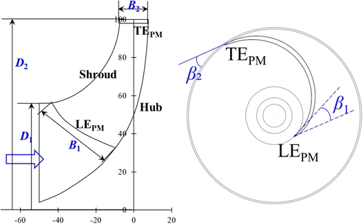
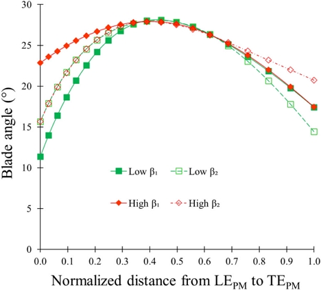
Fig. 1 indicates the meridional and plane views of the pump turbine impeller. The diameter of the impeller is designed to be D₁ = 112 mm for the scaled-down model test.^[13] The β₁ and β₂ are impeller blade inlet and outlet angles for the pump turbine in pump mode, respectively. Fig. 2 shows the impeller blade angle distribution from the leading edge to the trailing edge in pump mode. The performance and internal flow of the pump turbine according to the β₁ and β₂ are examined. The blade outlet angle was fixed at β₂ = 18° and the inlet angle was varied. Similarly, for the change in the impeller outlet angle β₂, the inlet angle was fixed at β₁ = 15°, and the outlet angle was varied. The three kinds of low, medium, and high blade angle distributions for β₁ and β₂, respectively, are selected for the design of the pump turbine impeller.

Fig. 1.

Meridional (left) and plane (right) views of pump turbine impeller in pump mode

Fig. 2.

Blade angle distribution of impeller at hub in pump mode

2.2 Numerical Methodology

The commercial code of ANSYS 2024R1^[14] is used for the computational analysis of pump turbines in pump and turbine modes. ANSYS CFX 2024R1^[14] uses Reynolds Averaged Navier Stokes (RANS) equations to solve the steady incompressible simulation with a shear stress transport (SST) turbulence model. The SST model combines the capabilities of the κ-ε model away from the walls and the robustness of the κ-ω turbulence model near the walls by blending functions. The SST model was designed to give highly accurate predictions of the onset and the amount of flow separation under adverse pressure gradients by transport effects into the formulation of the eddy viscosity. A large number of studies were carried out for the validation of the SST model.^[15] The SST model is appropriate for evaluating the flow at high rotation speed, especially in pumps and turbines.^[16] The hexahedral numerical grids are suitable for the proper and stable CFD analysis. ANSYS ICEM 2024R1^[14] is used to create the hexahedral numerical grids with a y⁺ < 10. The SST turbulence model with automatic wall treatment was applied for CFD analysis. The automatic wall treatment provides a better near-wall behavior of the turbulent quantities.^[17]

The SST with automatic near-wall treatment allows the smooth shift from a low Reynolds form to a wall function formulation. Therefore, the 1 < y⁺ < 100 range of y⁺ is preferable for SST with automatic near-wall treatment to conduct CFD analysis.

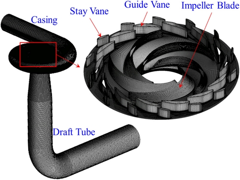
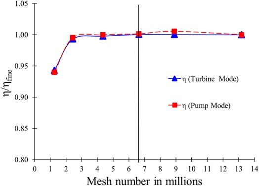
Fig. 3 shows the numerical grids of the pump turbine model. The mesh dependency test was conducted to obtain the suitable mesh number for CFD analysis. The mesh dependency test result is shown in Fig. 4. A 6.7 million node number is selected for the CFD analysis from the mesh dependency test. The detailed boundary conditions are shown in Table 1.

Fig. 3.

Numerical grids for pump turbine model

Fig. 4.

Mesh dependency test for medium β1 pump turbine at Q/QBEP=1.0

Table 1.

Boundary conditions for numerical analysis

3. Results and Discussion

3.1 Performance Curves of Pump Turbine

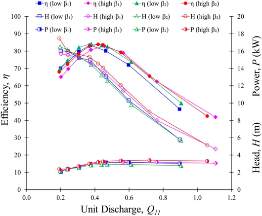
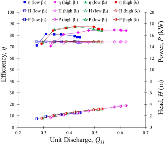
The performance curves of the pump turbine in pump and turbine modes with leakage flow are shown in Figs. 5 and 6, respectively. The unit quantities are used to compare the performance curves of the pump turbine.

N 11 = N D 1 H

(3)

Q 11 = Q D 12 H

(4)

P 11 = P ρ D 12 H 1.5

(5)

Fig. 5.

Performance curves of pump turbine model in pump mode according to β1 and β2 variation

Fig. 6.

Performance curves of pump turbine model in turbine mode according to β1 and β2 variation

The performance curves were evaluated in the pump mode of the pump turbine according to β₁ and β₂ variation. Fig. 5 shows the best efficiency of 84% matches the design point for low and high β₁ and β₂. At Q₁₁ =0.37, pump mode efficiencies are 83%, 81%, 84% and 83%, for low β₁, high β₁, low β₂ and high β₂, respectively. The best efficiencies of pump mode match the design point. At partial flow rate Q₁₁ = 0.20, the pump mode efficiencies are 65% and 68% for high β₁ and β₂, respectively. The pump turbine impeller with low β₁ and β₂ achieved 70% efficiency in pump mode. At the high flow rate, the performance of low β₁ is comparatively lower than others. At Q₁₁ = 0.20 and 0.90, the pump efficiency is decreased by 7% and 10% with a change in β₁ from low to high values, respectively. The pump mode efficiency decreased and increased by 2% and 9% with a change in β₂ from low to high values at Q₁₁ = 0.20 and 0.90, respectively.

Fig. 6 shows the performance curves of the pump turbine in turbine mode. The best efficiencies of low β₁ and high β₁ are 81% and 85% at Q₁₁ = 0.37 and 0.58, respectively. It indicates that turbine mode performance curves change drastically with β₁ variation. The high value of β₁ shows better performance in the turbine mode. The best efficiency in turbine mode is achieved at Q₁₁ = 0.42 for high and low β₂, respectively. The turbine mode efficiency for low and high β₂ is 87%.

3.2 S-Curve of Pump Turbine Model

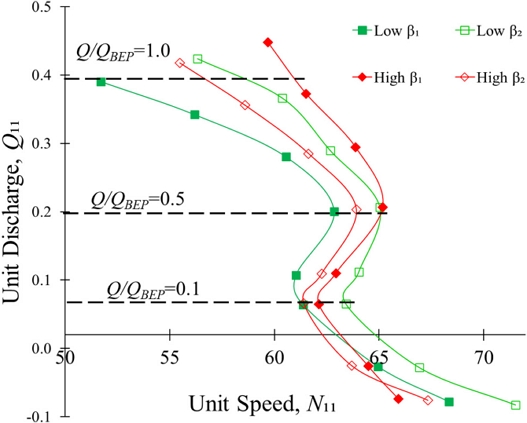
The hydraulic losses in the turbine mode at partial flow rates induce the S-Curve characteristic in the pump turbine. The S-Curve occurs in the turbine mode when the speed-discharge curve has a positive slope. The S-Curves are prepared by changing the flow rate at the constant guide vane opening.

Fig. 7 shows the S-Curve region of the pump turbine with the variation of β₁ and β₂. The S-Curve is prominent when the pump turbine operates at Q/Q_BEP < 0.5. The S-Curve begins from Q₁₁ = 0.18 and 0.19, and N₁₁ = 62.85 and 64.17, and ends at Q₁₁ = 0.09 and 0.04, and N₁₁ = 61.03 and 62.13 for low and high β₁, respectively. The S-Curve starts at Q₁₁ = 0.19 and 0.18, and N₁₁ =65.01 and 63.93, and the endpoints are N₁₁ = 63.41 and 61.94, and Q₁₁ = 0.05 for low and high β₂ pump turbines.

Fig. 7.

S-Curves of pump turbine according to β1 and β2

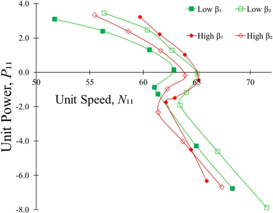
Fig. 8 shows the variation of P₁₁ vs N₁₁ according to the variations of β₁ and β₂. P₁₁ = 0 indicates zero power output condition in the pump turbine, which is a runaway speed condition. The runaway speeds for low and high β₁ are 62.81 and 65.12, and for low and high β₂ are 65.03 and 63.93, respectively.

Fig. 8.

P11 vs N11 characteristic curves of pump turbine according to β1 and β2

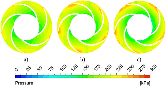
Fig. 9 shows pressure contours with a medium β₁ in the S-Curve range at the turbine mode of the pump turbine. The pressure contours indicate that, at the Q/Q_BEP = 0.5 and 0.1, the intense pressure rise is observed at the blade inlet in turbine mode. With a decreasing flow rate, a sudden rise in pressure at the blade inlet in turbine mode is observed.

Fig. 9.

Pressure contours in S-Curve range of pump turbine with medium β1 at Q/QBEP = a) 1.0, b) 0.5 and c) 0.1 in turbine mode

3.3 Loss Analysis in S-Curve Region

The hydraulic losses of the pump turbine in turbine mode include losses in the casing, stay vane, guide vane, impeller, and draft tube. Eq. (6) shows the turbine mode equation for the pump turbine. The objective of the study is to analyze losses in impellers.

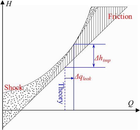
Fig. 10 shows the theoretical losses of the pump turbine impeller in turbine mode. As fluid passes through the impeller, it is subjected to hydraulic losses and leakage flow, and ideal energy transfer is not achieved. Shock and friction losses are dominant at a partial and high flow rate. Eq. (7) shows the main loss components in the pump turbine impeller in turbine mode, which includes shock and friction losses.^[19] The flow losses and throttling differences at various guide vane openings are considered for the pump turbine equation.^[19] The pump turbine equations using hydraulic losses are expressed by Eqs. (8)-(16).^[19]

Fig. 10.

Pump turbine performance difference in turbine mode including hydraulic losses[18]

h c + h s v + h g v + h i m p + h d + η h H = H

(6)

h s + h f = h i m p

(7)

a ϕ 22 - 2 b ϕ 2 k m 2 + c k m 2 2 + d k m 2 + e ϕ 2 - f = 0

(8)

k m 2 = Q π D 2 B 2 2 g H

(9)

ϕ 2 = π D 2 N 60 2 g H

(10)

a = ζ s + ζ u - 2 D 2 D 1 2

(11)

b = ζ s c o t α 2 + c o t β 2 + ζ u - 1 B 2 B 1 c o t β 1 - c o t α 2

(12)

c = ζ s c o t α 2 + c o t β 2 2 + ζ u c o t 2 β 1 + ζ f s e c 2 β 1 + ζ m × D 2 B 2 D 1 B 1 2

(13)

d = ϕ 2 n sin ⁡ α n - α 2 sin β 2 c o t α 2 + B 2 B 1 c o t β 1

(14)

e = k m 2 n sin β 2 c o t α 2 + B 2 B 1 c o t β 1

(15)

f = sin β 2 sin ⁡ α n - α 2 + 1 c o t α 2 + B 2 B 1 c o t β 1 × ϕ 2 n k m 2 n + 1

(16)

ϕⁿ and $k m n$ are values at the rated operating points.

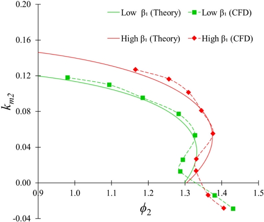
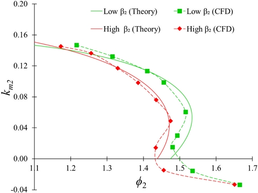
The coefficient of the equation is dependent on the impeller blade angle, which is related to the loss components. The coefficients a, b, and c are related to shock and friction losses in the impeller. The d, e, and f coefficients are related to the throttling difference between guide vane openings. The study objective is to evaluate the impeller losses in the S-Curve region. S-Curves were prepared using CFD analysis. Figs. 11 and 12 show the comparison between theoretical and CFD analysis results for β₁ and β₂ variation at α = 17° and 21°, respectively. The curve-fitting regression methodology is applied to calculate Eq. (8) coefficients from CFD analysis. The losses in the casing, stay vane, guide vane, and draft tube are neglected, letting ζ_m = 0 and ζ_u = 1. The shock and friction loss coefficients were calculated by solving Eqs. (11)-(16).

Fig. 11.

S-Curve according to β1 by loss analysis at α=17

Fig. 12.

S-Curve according to β2 by loss analysis at α=21°

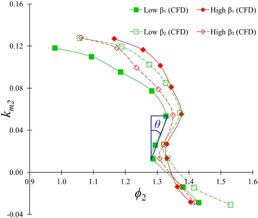
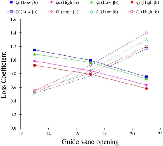
Fig. 13 shows the S-Curve comparison according to β₁ and β₂. S-Curve inclination is measured to evaluate the steepness of the S-Curve. The S-Curve inclination for low β₁ and high β₂ are 24° and 22°, respectively. It implies that β₁ variation has minimum influence in an S-Curve inclination. The S-Curve inclination decreased from 26° to 15° when β₂ increased from 14° to 20°. Fig. 14 shows the variation of the shock and friction loss coefficient according to β₁ and β₂ in the S-Curve region. The shock and friction loss coefficient decreases and increases with an increase in guide vane opening. At α =13°, the low β₁ and high β₂ showed the maximum and minimum shock loss coefficient. At α =13°, the shock loss coefficient is decreased by 14% and 15% with an increase in β₁ and β₂ from low to high value, respectively. When β₁ and β₂ increase from low to high values, the shock loss coefficient is reduced by 16% and 19%, respectively, at α = 21°. At α = 13°, the friction loss coefficient value is approximately the same for every β₁ and β₂ value. At α = 21°, the maximum friction coefficient value is 1.4 for high β₁. The friction coefficient value is increased and decreased by 20% and 8% with an increase in β₁ and β₂ from low to high value, respectively, at α = 21°. The loss analysis showed that the shock loss coefficient decreases with an increase in β₁ and β₂. The friction loss coefficient decreases with a decrease in β₁ and an increase in β₂. The loss analysis showed that high β₂ has comparatively a lower shock and friction loss coefficient value.

Fig. 13.

S-Curve according to β1 and β2 by loss analysis at α=17°

Fig. 14.

Loss coefficient in impeller according to β1 and β2 in S-Curve region

4. Conclusion

The low specific speed pump turbine was selected for the current study. The impeller blade profile changes according to β₁ and β₂. The influence of β₁ and β₂ on the performance and flow behavior of the pump turbine were evaluated independently by CFD analysis. The best efficiency of the pump turbine in pump mode is higher than 80% for all the cases. At high flow conditions, low β₁ and β₂ showed comparatively lower efficiency. The best efficiency of the pump turbine in turbine mode is 81% and 85% for low and high β₁ at Q₁₁ = 0.31 and 0.58, respectively. The best efficiency for the pump turbine in turbine mode is 87% with low and high β₂. The S-Curve inclination is reduced from 26° to 15° with an increase in β₂ from 14° to 20°. The shock and friction loss coefficients increase and decrease with an increase in the guide vane opening. The shock and friction loss is maximum for low and high β₁ at α = 13° and 21°. The increase in β₂ value reduces the S-Curve inclination, shock and friction loss coefficients in the turbine mode operation of the pump turbine.

Nomenclature


B :	impeller width (m)
D :	impeller diameter (m)
H :	effective head (m)
LE :	leading edge
N :	rotational speed (min^-1)
P :	power (kW)
Q :	flow rate (m³/s)
TE :	trailing edge
h :	hydraulic loss
k_m :	meridian velocity coefficient
n_sp :	specific speed
Δq_leak :	leakage flow
α :	guide vane opening angle
β :	blade angle
ζ_s :	shock loss coefficient
ζ_f :	friction loss coefficient
ζ_m :	loss coefficient of meridian velocity
ζ_u :	loss coefficient of circumferential velocity
η_h :	hydraulic efficiency
θ :	S-Curve inclination
ρ :	density (kg/m³)
ω :	rotational speed (rad/s)
ϕ :	circumferential velocity coefficient

Subscript


1 :	inlet in pump mode
2 :	outlet in pump mode
11 :	unit quantities
c :	casing
d :	draft tube
gv :	guide vane
imp :	impeller
sv :	stay vane
s :	shock loss
f :	friction and mixing loss in impeller passage
PM :	pump mode
TM :	turbine mode

References

Simão, M., and Ramos, H.M., 2020, “Hybrid pumped hydro storage energy solutions towards wind and PV integration: Improvement on flexibility, reliability and energy costs”, Water, 12(9), 2457. [https://doi.org/10.3390/w12092457]
Vasudevan, K.R., Ramachandaramurthy, V.K., Venugopal, G., Ekanayake, J.B., and Tiong, S.K., 2021, “Variable speed pumped hydro storage: A review of converters, controls and energy management strategies”, Renew. Sustain. Energy Rev., 135, 110156. [https://doi.org/10.1016/j.rser.2020.110156]
Cavazzini, G., Covi, A., Pavesi, G., and Ardizzon, G., 2016, “Analysis of the unstable behavior of a pump-turbine in turbine mode: Fluid-dynamical and spectral characterization of the S-shape characteristic”, J. Fluids Eng., 138(2), 021105. [https://doi.org/10.1115/1.4031368]
Zuo, Z., Fan, H., Liu, S., and Wu, Y., 2016, “S-shaped characteristics on the performance curves of pump-turbines in turbine mode–A review”, Renew. Sustain. Energy Rev., 60, 836-851. [https://doi.org/10.1016/j.rser.2015.12.312]
Cavazzini, G., Covi, A., Pavesi, G., and Ardizzon, G., 2015, “Numerical analysis of the S-shape characteristic in a pump-turbine”, Proc. 11^th European Conference on Turbomachinery Fluid dynamics & Thermodynamics, European Turbomachinery Society.
Casartelli, E., Del Rio, A., Mangani, L., and Schmid, A., 2022, “Capturing the S-shape of pump-turbines by computational fluid dynamics simulations using an anisotropic turbulence model”, J. Fluids Eng., 144(2), 021203. [https://doi.org/10.1115/1.4051809]
Ji, Q., Wu, G., Liao, W., and Fan, H., 2022, “Flow deflection between guide vanes in a pump turbine operating in pump mode with a slight opening”, Energies, 15(4), 1548. [https://doi.org/10.3390/en15041548]
Wang, L., Zhang, K., and Zhao, W., 2022, “Nonlinear modeling of dynamic characteristics of pump-turbine”, Energies, 15(1), 297. [https://doi.org/10.3390/en15010297]
Zhang, F., Fang, M., Tao, R., Liu, W., Gui, Z., and Xiao, R., 2023, “Investigation of energy loss patterns and pressure fluctuation Spectrum for pump-turbine in the reverse pump mode”, Journal of Energy Storage, 72(Part A), 108275. [https://doi.org/10.1016/j.est.2023.108275]
Deng, Y., Xu, J., Li, Y., Zhang, Y., and Kuang, C., 2022, “Experimental and computational fluid dynamics study of the flow field of a model pump turbine”, Front. Energy Res., 10, 911874. [https://doi.org/10.3389/fenrg.2022.911874]
Wang, H., Wang, J., Gong, R., Shang, C., Li, D., and Wei, X., 2021, “Investigations on pressure fluctuations in the S-shaped region of a pump–turbine”, Energies, 14(20), 6683. [https://doi.org/10.3390/en14206683]
Zanetti, G., Cavazzini, G., and Santolin, A., 2023, “Three-dimensional evolution of the flow unsteadiness in the S-shape of pump-turbines and its correlation with the runner geometry”, Journal of Energy Storage, 57, 106176. [https://doi.org/10.1016/j.est.2022.106176]
Shrestha, U., Singh, P.M., and Choi, Y-D., 2019, “Design and experimental analysis on 3kW class pump turbine model for renewable ESS”, The KSFM Jounral of Fluid Machinery, 22(4), 19-28. [https://doi.org/10.5293/kfma.2019.22.4.019]
ANSYS Inc., 2024, “ANSYS CFX documentation version 2024R1”, http://www.ansys.com, .
Bardia, J. E., Huang, P.G., and Coakley, T.J., 1997, “Turbulence modeling validation, testing and development”, NASA, California. [https://doi.org/10.2514/6.1997-2121]
Zhao, W., and Zhao, G., 2018, “Numerical investigation on the transient characteristics of a sediment-laden two-phase flow in a centrifugal pump”, Journal of Mechanical Science and Technology, 32(1), 167-176. [https://doi.org/10.1007/s12206-017-1218-6]
Erne, S., Edinger, G., Maly, A., and Bauer, C., 2017, “Simulation and experimental investigation of the stay vane channel flow in a reversible pump turbine at off-design conditions”, Period. Polytech. Mech. Eng., 61(2), 94-106. [https://doi.org/10.3311/PPme.9345]
Chapallaz, J.M., Eichenberger, P., and Fischer, G., 1992, “Manual on pumps used as turbines”, Skat, Denmark.
Xia, L., Cheng, Y., You, J., Zhang, X., Yang, J., and Qian, Z., 2017, “Mechanism of the S-shaped characteristics and the runaway instability of pump-turbines”, J. Fluids Eng., 139(3), 031101. [https://doi.org/10.1115/1.4035026]

Specification	Turbine Mode	Pump Mode
Inlet	Total Pressure	Static Pressure
Outlet	Static Pressure	Mass Flow Rate
Turbulence Model	Shear Stress Transport
Interface Model	Frozen Rotor
Wall Condition	No Slip Wall