Wave Analysis Method for Offshore Wind Power Design Suitable for Suitable for Ulsan Area

1. Introduction

With the recent acceleration of global warming caused by carbon emissions, various such as sea-level rise, extreme droughts, ecosystem destruction, and reduced crop production have become serious concerns. In response, various industries are focusing their efforts on reducing carbon emissions. The energy sector, traditionally reliant on sources like coal, oil, and nuclear power, is transitioning rapidly towards renewable energy. Wind power generation, with its high technological maturity and economic feasibility, is gaining attention as an effective option for reducing carbon emissions.^[1]

Compared to land-based wind power generation, OWPG offers numerous advantages, including excellent wind resources and energy generation, ease in developing large-scale wind farms, landscape preservation, and reduced noise. Consequently, a global expansion of OWPG technology is underway.^[2] South Korea is also gradually transitioning from land-based wind farms to offshore wind farms. Initiatives include the construction of a 30 MW fixed offshore wind turbine off the northwest coast of Jeju in September 2017 and the completion of a 60 MW offshore wind turbine testbed in the southwest sea in January 2020.

In the ongoing project for Korea’s offshore wind farm construction, Jeonnam is advancing an 8.2 GW fixed offshore wind project by 2030. Meanwhile, in Ulsan, multiple global turbine companies and developers are collaborating on a plan to construct a 6 GW floating offshore wind farm off the east coast of Korea.^[3]

The construction of wind farms involves several steps, including analyzing marine environmental conditions, predicting the wind power generation capacity, selecting a wind turbine class, and determining design conditions for the wind farm layout and turbine system. Floating offshore wind turbines, unlike fixed ones, require consideration of various external load conditions such as waves, currents, and wind, as they directly impact the turbine system and floating structure’s operation and viability. Thus, the collection and analysis of data related to marine environmental conditions are integral components in the construction of offshore wind farms.

Marine environment data, including information on wind, marine conditions, climate, and seabed conditions required for the design of a floating offshore wind turbine system, should be analyzed in accordance with international standards such as IEC61400-3, DNV RP, and ABS.^[4]

Marine environment data can be collected as meteorological data from offshore meteorological towers and floating LiDAR equipment. Moreover, to estimate the extreme value of marine conditions with a high reliability using statistical analysis methods, an amount of data corresponding to 1/4 of the return period must be available.^[5] However, it is almost impossible to maintain a high recovery rate while monitoring long-term data under extreme marine environment conditions. Accordingly, in recent years, many researchers have used numerical methods to obtain long-term data such as hindcast.

Sheridan et al. (2020) conducted a comparative validation between data collected by two floating LiDAR off the coasts of California, New Jersey, and Virginia and five sets of reanalysis data (MERRA-2, CFSv2, NARR, and RAP) to demonstrate that the ERA5 and RAP models were the most reliable with the lowest wind speed deviation and highest correlation at near surface and hub heights 50-100 m level.^[6~13]

Sharmar and Markina (2020) used WAVE WATCH III, a numerical wave model, and various reanalysis wind field models (ERA5, ERA-Interim, NCERP CFSR, and MERRA-2) to validate the reliability of hindcast data. The study compared data collected from offshore buoys and hindcast data generated by various wind field models based on statistical error indices (i.e., normalized bias, scatter index, and root mean square error) and reported that the data generated by ERA5-Wave WATCH III were most similar to actual measured values.^[14]

Jeong et al. (2016) generated hindcast data in Korean Seas using the SWAN numerical wave model through applying the ECMWF wind field data and conducted a comparative analysis study that compared these data to annual average and peak Hs observation data of the corresponding areas. In that study, Hs time series data were in relatively close agreement and demonstrated a high correlation, but the peak value of hindcast data in high wave areas tended to be under-predicted.^[15]

To enhance the quality of hindcast data, it is important to select and apply the wind field model based on whether the objective of the study is a global or regional climate assessment. If it is the latter, a prediction model that can model the climate of the region at high resolution should be used. Recently the KIOST also generated hindcast data suitable for Korean waters using the SWAN numerical wave model and high-resolution WRF wind field model, and Jeong et al. (2016) and Eum et al. (2020) conducted validation studies on numerical hindcast data model for analyzing marine environment conditions.^[15,16] The reliability of the generated hindcast data was validated through a comparison and review against observational data from offshore buoys operated by the KHOA, MOF and KMA; a hindcast database for all Korean sea areas was established based on this approach.

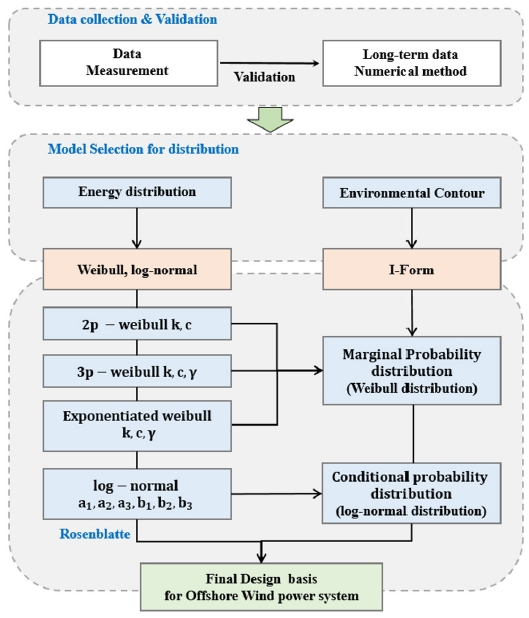
As shown in Fig. 1, the procedures for analyzing external environmental conditions consist of data collection and validation, distribution function model selection, estimation of the parameters of the applicable model, and an analysis of environmental conditions. Up to present, most researchers have used the Weibull distribution, which has characteristics similar to an energy distribution with a low frequency of extreme values and high frequency of low values, when analyzing the marine environment. Weibull distributions can be divided into 2p, 3p, and exponentiated Weibull distributions according to the composition of parameters, and recently, Pobočíková et al. (2023) compared the characteristics of these distributions based on wind data from the Poprad region in Slovakia. The wind data were compared by months and seasons using six types of GOF testing methods, and the study results indicated that the exponentiated Weibull distribution was most similar to the collected wind data as it provided relatively high flexibility.^[17]

Fig. 1.

A procedure for analyzing external environmental conditions

The Gumbel function and I-FORM are widely used as the main methods for estimating extreme values. The Gumbel function is used to estimate the extreme value of a single variable, whereas I-FORM is used to estimate the extreme value of two or more combined variables. More specifically, with I-FORM, marine conditions with combinations of various external conditions acting on them can be combined to be expressed as a limit state. Accordingly, international standards such as IEC61400-3 Annex G, DNVGL-RP-C205, and NORSOK actively recommend the use of I-FORM in OWP turbine system design. The Gumbel function and I-FORM have the same purpose of use for extreme value estimation. However, as shown in Fig. 1, I-FORM differs in that it considers two or more variables to represent a critical limit state and design point.

Recently, Park et al. (2020) used wind, wave, and current data collected from the Barents Sea hindcast data to estimate the parameters of 2p and 3p Weibull distributions, which were then used to perform EVA using I-FORM. EVA using the parameters of the 2p Weibull distribution showed values similar to the collected data, but that of the 3p Weibull distribution showed overestimated results.^[18]

An existing study by Pobočíková et al. (2023) reported that the exponentiated Weibull distribution was the most suitable model under normal wind conditions, but the study did not perform an additional analysis under extreme wind conditions. Moreover, the extreme condition analysis study by Park et al. (2020) presented analysis results that evaluated only the 2p and 3p Weibull distributions, and not the exponentiated Weibull distribution.

In the present study, marine environment data from the Ulsan sea area in Korea were used to calculate return period values necessary for designing floating OWP systems. The data collected from a marine meteorological buoy comprised short-term data spanning six years. However, due to insufficient quantity, these data were not suitable for use in EVA. Therefore, long-term hindcast data were employed instead and validity of the data was confirmed by comparing hindcast data with measured data from buoys. The parameters of the Weibull distribution were estimated using LSM, and checked for reliability by comparison with the CDF of the measured data. To derive a method suitable for extreme condition analysis in the Ulsan sea area of South Korea, this study additionally included the exponentiated Weibull distribution, which was not previously considered in the study conducted by Park et al. (2020).

This study proposes the most appropriate Weibull distribution model for extreme value analysis. This is demonstrated by comparing the error rates between the maximum value observed in the hindcast data and the estimated extreme values. Through this comprehensive procedure, we provide the extreme values of Hs and Tp that are essential for the accurate design of an offshore wind system in the waters off Ulsan, Korea.

2. Marine environment data

2.1 Collection of marine environment observation data

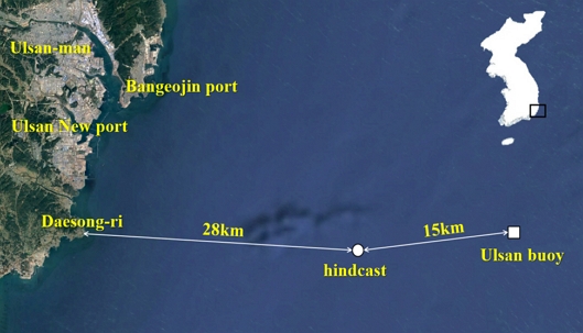
Marine environment observation data were acquired over a six years period (January 1, 2016 to December 31, 2021) using a marine meteorological buoy operated by KMA. The marine meteorological buoy is located at 35°20′43.00″N, 129°50′29.00″E, approximately 43 km off the coast of Daesong-ri, Ulsan. This location is suitable for acquiring marine environment data because there is no interference from nearby topography, landmarks, and reefs. Detailed information about the site coordinate, instrument, data recovery rate, monitoring period, measurement time interval, and observed items is provided in Table 1.

Table 1.

Marine environment buoy monitoring conditions

2.2 Marine environment hindcast data collection

KIOST has generated hindcast data using a WRF wind field and SWAN numerical wave model that includes wind-induced wave generation, wave dissipation, three-wave nonlinear interactions, and four-wave nonlinear interactions. In the present study, data from hindcast database developed by KIOST were used for comparison and validation against the buoy observation data. The location had coordinates of 35°19′58.78″N, 129°40′1.17″E, which is approximately 15 km from the buoy. Detailed information is given in Table 2 and Fig. 2.

Table 2.

Marine environment monitoring condition of hindcast data

Fig. 2.

Locations of observation buoy and hindcast data

2.3 Data Validation

The wind speed and Hs observation data collected by the marine meteorological buoy between 2016 and 2021 and hindcast data for the same period were compared and analyzed to test the validity of the data. The characteristics of the hindcast data were reviewed using a time series validation and the hourly and daily R² and error metrics were calculated to quantitatively analyze the accuracy between the model estimated values and observed values. Typical error metrics include bias, MAE, CRMS, and RMSE, which can be defined by Eq.(1)-(4) as follows:^[19]

$\[ \text{ Bias }=\frac{1}{\mathrm{N}}{\mathrm{\Sigma }}_{\text{i}=1}^{\text{N}}\left({\mathrm{V}}_{\text{mod},i}-V_{obs,i}\right) \]$

(1)

$\[ \mathrm{M}\mathrm{A}\mathrm{E}=\frac{1}{\mathrm{N}}{\Sigma }_{\text{i}=1}^{\text{N}}\left|{\mathrm{V}}_{\text{mod},i}-V_{obs,i}\right| \]$

(2)

$\[ \text{CRMSE }=\sqrt{\frac{1}{\mathrm{N}}{\mathrm{\Sigma }}_{\text{i}=1}^{\text{N}}{\left[\left({\mathrm{V}}_{\mathrm{m}\mathrm{o}\mathrm{d},\mathrm{i}}-\overline{{\mathrm{V}}_{\mathrm{m}\mathrm{o}\mathrm{d}}}\right)-\left({\mathrm{V}}_{\mathrm{o}\mathrm{b}\mathrm{s},\mathrm{i}}-\overline{{\mathrm{V}}_{\mathrm{o}\mathrm{b}\mathrm{s}}}\right)\right]}^2} \]$

(3)

$\[ \mathrm{R}\mathrm{M}\mathrm{S}\mathrm{E}=\sqrt{\frac{1}{\mathrm{N}}{\mathrm{\Sigma }}_{\text{i}=1}^{\text{N}}{\left({\mathrm{V}}_{\mathrm{m}\mathrm{o}\mathrm{d},\mathrm{i}}-{\mathrm{V}}_{\mathrm{o}\mathrm{b}\mathrm{s},\mathrm{i}}\right)}^2} \]$

(4)

where, N is the number of data points; Vmod and Vobs represent estimates from the hindcast data and buoy-observed values, respectively, and $$ \overline{{\mathrm{V}}_{\mathrm{m}\mathrm{o}\mathrm{d}}}$$ and $$ \overline{{\mathrm{V}}_{\mathrm{o}\mathrm{b}\mathrm{s}}}$$ represent the mean value of each data. Bias indicates the mean deviation between the model estimate and observed value, MAE indicates the mean of all absolute errors of the estimates and observed values, RMSE indicates the mean root square of estimation error, and CRMSE indicates the difference in variation of the estimate and observed value based on the center of the error.

2.3.1 Validation of hindcast data characteristics

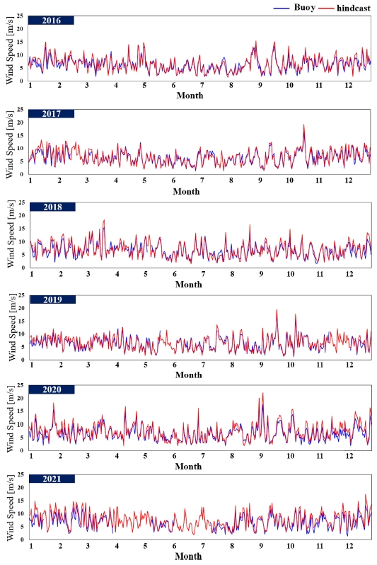
Fig. 3 shows the time series data for daily average wind speed of buoy-observed data and hindcast data collected at the same times between 2016 and 2021.

Fig. 3.

Time series of hindcast data wind speed and buoy-observed wind speed

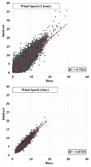
The results for the time series comparison of daily hindcast and observed data showed generally high similarity. However, the hindcast data values tended to show localized under- or over-estimation in some intervals, as compared to the observed values. To perform a more precise assessment of data reliability, hourly and daily wind speed data were quantitatively analyzed, and the results are shown in Table 3. The results of 1day average data show a relatively lower error rate as compared to 1hour raw data. These results were the product of errors, with the large local variability being offset as 1hour raw data were averaged. Fig. 4 shows the R² of the 1hour raw wind data and 1day average wind data. The probability of data occurrence over 15 m/s high wind speed intervals was relatively low, but the hindcast data values tended to be over-estimated relative to the observed values.

Table 3.

Error metric result of wind speed

Fig. 4.

Coefficients of determination (R2) of wind speed

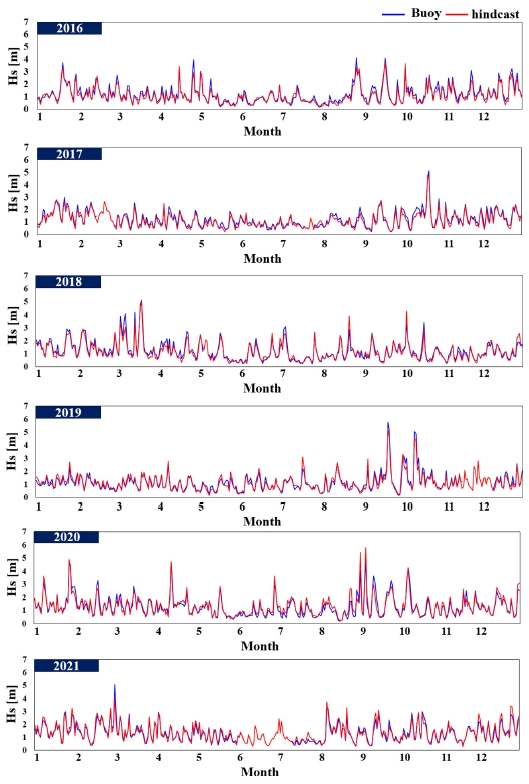
Fig. 5 shows the time series data for 1day average Hs from the observed and hindcast data collected during the same period between 2016 and 2021. Overall, the similarity of Hs data was high. In significant wave height under 3 m, the hindcast data values tended to be under-estimated during the entire observation period, except 2020. Table 4 shows the quantitative analysis results.

Fig. 5.

Time series of hindcast data Hs and buoy-observed Hs

Table 4.

Error metric result of wind speed

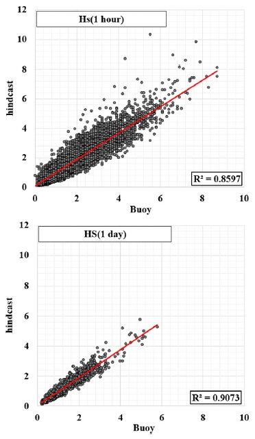
Fig. 6 shows the R² of 1hour Hs raw data and 1day Hs average data. These values demonstrated a similarity higher reliability as compared to the wind speed data.

Fig. 6.

Coefficients of determination (R2) of significant wave height

3. Statistical analysis methods

Probability distributions and parameters selected for statistical analysis may have a significant impact on the reliability of analysis of marine environment conditions. Energy sources such as waves, currents, and wind exhibit frequency distributions that closely resemble the Weibull distribution. Therefore, the Weibull distribution is widely used in the marine field to analyze environmental conditions. Moreover, because OWP and offshore structures exhibit external environmental characteristics that combine two or more variables (i.e., wind speed-turbulence intensity, wave height-wave period, and so on), estimating extreme values using I-FORM is recommended. For example, the wave height found at a specific wave period may be higher than the wave height found under the longest wave period condition; in such a case, the wave load generated at that wave period could have an even greater impact on the response of the structure.

3.2 Extreme value analysis of inverse first order reliability method

I-FORM, first proposed by Winterstein is an EC method that effectively approximates the limit state of a given return period.^[21] This method is used in various fields, including offshore structure design, natural disaster prediction, and environmental risk analysis. Eq. (12) shows the joint probability distribution of Hs and the peak period, which can be expressed as the product of marginal probability distribution of Hs and conditional probability distribution of corresponding peak period, respectively.

$\[ {\mathrm{f}}_{{\mathrm{H}}_{\mathrm{s}}{\mathrm{T}}_{\mathrm{D}}}\left({\mathrm{h}}_{\mathrm{S}},{\mathrm{t}}_{\mathrm{p}}\right)={\mathrm{f}}_{{\mathrm{H}}_{\mathrm{s}}}\left({\mathrm{h}}_{\mathrm{S}}\right){\mathrm{f}}_{{\mathrm{T}}_{\mathrm{D}}\left|{\mathrm{H}}_{\mathrm{s}}\right.}\left({\mathrm{t}}_{\mathrm{p}}|{\mathrm{h}}_{\mathrm{S}}\right) \]$

(12)

Where, f_Hs(h_s) is the marginal probability distribution of Hs, f_Tp|Hs(t_p|h_s) is the conditional probability distribution, HS is the significant wave height, and Tp is the peak period. Generally, f_Hs(h_s), the marginal probability distribution of Hs (assumed to be a Weibull distribution), can be defined by Eq. (13), whereas f_Tp|Hs(t_p|h_s), the conditional probability distribution of the peak period (assumed to be a log-normal distribution), can be defined by Eq. (14).

$\[ {\text{f}}_{{\text{H}}_{\text{s}}}\left({\text{h}}_{\text{S}}\right)=\frac{\text{k}}{\text{c}}{\left(\frac{{\text{h}}_{\text{s}}}{\text{c}}\right)}^{\text{k}-1}\text{exp}\left[-{\left(\frac{{\text{h}}_{\text{s}}}{\text{c}}\right)}^{\text{k}}\right] \]$

(13)

$\[ {\mathrm{f}}_{{\mathrm{T}}_{\text{p}}\left|{\mathrm{H}}_{\mathrm{s}}\right.}\left({\mathrm{t}}_{\mathrm{p}}|{\mathrm{h}}_{\mathrm{S}}\right)=\frac{1}{{\mathrm{t}}_{\mathrm{p}}\sigma \sqrt{2\pi }}\text{exp}\left[\frac{-{\left(\mathrm{l}\mathrm{n}\left({\mathrm{t}}_{\mathrm{p}}\right)-\mu \right)}^2}{2{\sigma }^2}\right] \]$

(14)

Where, k, c, μ, and σ² represent the shape parameter, scale parameter, mean, and variance, respectively, and when a 3p or exponentiated Weibull distribution is used on the marginal probability distribution, parameter γ or γ_EW is added.

Eq. (15) and (16) define parameters μ and σ² of the conditional probability distribution used in a log-normal distribution; these are determined by E[ln(t_p)] and VAR[ln(t_p)] corresponding to each interval of Hs. Parameters a1, a2, a3, b1, b2, and b3 are estimated by a non-linear fitting method.^[22]

$\[ \mu ={\mathrm{a}}_1+{\mathrm{a}}_2\cdot {\mathrm{h}}_{\mathrm{s}}^{{\mathrm{a}}_3} \]$

(15)

$\[ {\sigma }^2={\mathrm{b}}_1+{\mathrm{b}}_2\cdot \text{exp}\left[-{\mathrm{h}}_{\mathrm{s}}\cdot {\mathrm{b}}_3\right] \]$

(16)

I-FORM, based on the conventional structural reliability approach, is a method for determining the exceedance probability according to the return period and corresponding response level. All variables are independent and follow a Gaussian distribution. The order by which I-FORM is used to derive the contour line is as follows.^[23]

• [Step 1] The exceedance probability (P) of a given return period can be derived by Eq. (17).

$\[ \mathrm{P}\left[\mathrm{X}>\mathrm{x}\right]=1-\mathrm{F}\left(\mathrm{x}|\mu ,\sigma \right) \]$

(17)

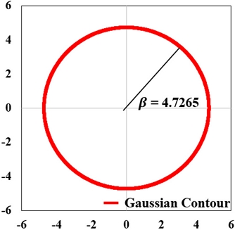
• [Step 2] The probability of condition P[X>x] can be derived by Eq. (18), whereas Eq. (19), representing an inversed Gaussian cumulative distribution, can be applied to derive the radius of U-space (β) with mean of 0 and standard deviation of 1, as shown in Fig. 7.

$\[ \mathrm{P}\left[\mathrm{X}>\mathrm{x}\right]=\mathrm{F}\left(\mathrm{x}|\mu ,\sigma \right) \]$

(18)

$\[ \beta =\mathrm{x}={\mathrm{F}}^{-1}\left(\mathrm{p}|\mathrm{0,1}\right) \]$

(19)

Fig. 7.

U-space of 100year return period

• [Step 3] Parameters of Weibull (k, c) and log-normal distributions (a₁, a₂, a₃, b₁, b₂, b₃) are estimated using Eq. (11), (15), and (16).

• [Step 4] Eq. (20) and (21), transformation formulas proposed by Rosenblatt, can be used to transform U-space into a physical parameter space, the target response level, is found as the highest value on the surface in the physical parameter space.^[24]

$\[ \mathrm{F}\left({\mu }_1\right)=1-\text{exp}\left[-{\left(\frac{{\mathrm{h}}_{\mathrm{s}}}{\mathrm{c}}\right)}^{\mathrm{k}}\right] \]$

(20)

$\[ \mathrm{F}\left({\mu }_2\right)=\frac{1}{2}+\frac{1}{2}erf\left[\frac{\mathrm{l}\mathrm{n}\left(t_p\right)-\mu \left(h_s\right)}{\sqrt{2\sigma \left(h_s\right)}}\right] \]$

(21)

h_s can be defined by Eq. (22)-(24) depending on the parameters that comprise the Weibull distribution, whereas T_p corresponding to h_s can be defined by Eq. (25).

$\[ {\mathrm{h}}_{\mathrm{s}\left(2\mathrm{p}\text{ Weibull}\right)}=\mathrm{c}{\left[-\mathrm{l}\mathrm{n}1-\mathrm{F}\left({\mu }_1\right)\right]}^{\frac{1}{\mathrm{k}}} \]$

(22)

$\[ {\mathrm{h}}_{\mathrm{s}\left(3\mathrm{p}\text{ Weibull}\right)}=\mathrm{c}{\left[-\mathrm{l}\mathrm{n}1-\mathrm{F}\left({\mu }_1\right)\right]}^{\frac{1}{\mathrm{k}}}+\gamma \]$

(23)

$\[ {\mathrm{h}}_{\mathrm{s}\left(\text{Exponentiated}\right)}=\mathrm{c}{\left[-\mathrm{l}\mathrm{n}1-\mathrm{F}{\left({\mu }_1\right)}^{\frac{1}{{\gamma }_{\mathrm{E}\mathrm{W}}}}\right]}^{\frac{1}{\mathrm{k}}} \]$

(24)

$\[ {\mathrm{t}}_{\mathrm{p}}=\text{exp}\left[\left(\sqrt{\sigma \cdot {\mu }_2}\right)+\mu \right] \]$

(25)

μ and σ² of the conditional probability distribution can be derived by Eq. (15) and (16).

The methods for extracting data used in I-FORM can be divided into the global approach, which uses all data measured over a long period, and the event approach, which extracts only data that exceed a certain.^[25] The hindcast data used in the present study represent 43years of data, and because there was sufficient data, the global approach was chosen.

4. Extreme wave condition analysis of East Sea of Korea

Floating OWP systems that are exposed to various external environmental conditions require a system optimization design that incorporates the site characteristics, including wind, waves, and currents. Wave conditions can prominently cause stress and fatigue load on the floating structure and act as a key factor that determines the dynamic response and motion performance of the structure. Accordingly, international standards, such as DNV-GL and ABS, recommend that the I-FORM statistical approach should be used for designing offshore structures to incorporate the extreme values of Hs for a return period of 100years and corresponding Tp in the design. An estimation of incorrect extreme value can cause the under- or over-design of an offshore structure, which can have a negative impact on its structural integrity and economic feasibility. Accordingly, to assure the reliability of extreme value estimation, a series of extreme wave analyses was conducted with various Weibull distribution models applied to I-FORM.

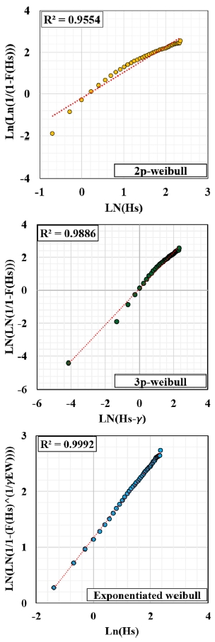
Fig. 8 shows the results from estimating the parameters of 2p, 3p, and exponentiated Weibull distributions using LSM. The exponentiated Weibull distribution and hindcast data were in close accordance. The parameter results are shown in Table 5.

Fig. 8.

Coefficients of determination of significant wave height for Weibull distribution parameters

Table 5.

Parameters for Weibull distribution

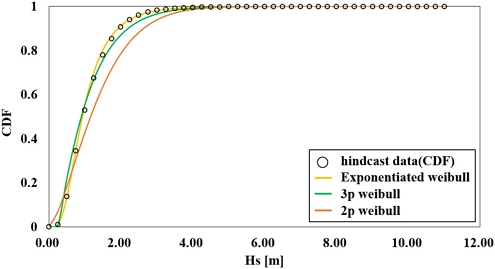
The CDF were compared to verify the estimated values of the parameters. The results of which are shown in Fig. 9. The exponentiated Weibull CDF closely resembled hindcast data at all intervals, whereas the 3p Weibull distribution showed similar results in some intervals between Hs greater than or equal to 1m and less than or equal to 1.5 m. In contrast, the 2p Weibull distribution showed over-estimations in intervals between Hs greater than or equal to 0 m and less than or equal to 0.5 m and under-estimations in intervals of Hs greater than 0.5 m, with slight differences in all intervals.

Fig. 9.

CDF of hindcast data and each Weibull distribution

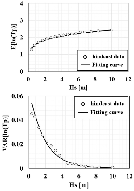
The conditional probability distribution applied in I-FORM was determined by E[ln(t_p)] and VAR[ln(t_p)] of Tp corresponding to Hs. The distribution of Hs typically demonstrated high frequency and narrow scatter in low-wave intervals, and thus, it was important to reproduce the distribution characteristics by setting the bin spacing to be small. Accordingly, the bin of Hs was set to 0.25 m, and the [ln(t_p)] and VAR[ln(t_p)] of Tp corresponding to this value were calculated. Parameters a₁, a₂, a₃, b₁, b₂, and b₃ were derived by non-linear fitting using Eq. (15) and (16), the results of which are shown in Table 6 and Fig. 10.

Table 6.

Estimation of conditional probability distribution parameters

Fig. 10.

Estimation of conditional probability distribution parameters

The error rates of peak Hs of hindcast data and estimated extreme values were calculated to validate the reliability of the I-FORM EVA results. Relative to the peak Hs value of hindcast data, EVA results larger than that value were expressed as “+” and results smaller than that value were expressed as “-,” as shown in Table 7.

Table 7.

Comparison of extreme values (I-form vs hindcast data)

The results from I-FORM EVA using the parameters of the exponentiated Weibull distribution overestimated Tp. However, the error rates of Hs and Tp were within 5%, showing a higher accuracy than the 2p and 3p Weibull distributions. The results from I-FORM EVA using the parameters of the 2p and 3p Weibull distributions underestimated Hs and Tp as compared to hindcast data, whereas Hs showed a large error rate of at least 10%.

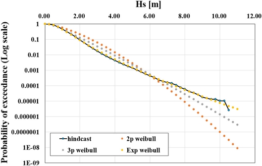
Fig. 11 represents the results of each probability of exceedance on a log scale, demonstrates the the exponentiated Weibull distribution has the best agreement with the hindcast, indicating the highest reliability in the I-FORM estimation results. Based on such findings, the exponentiated Weibull distribution was confirmed to most accurately reproduce the extreme value distribution characteristics of waves and is identified as the most suitable model for EVA.

Fig. 11.

Comparison on probability of exceedance (Log sacle)

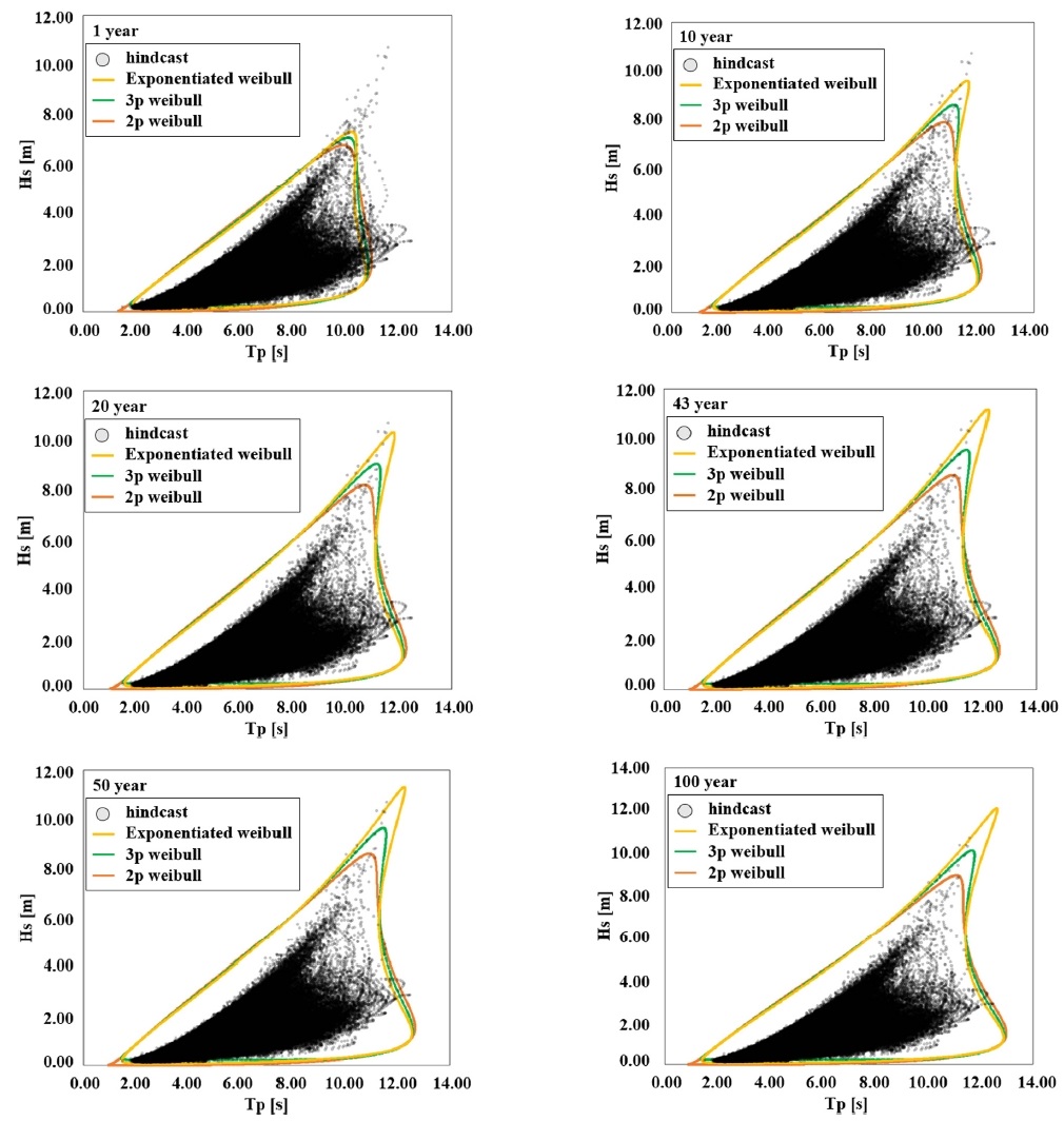
Fig. 12 shows the contour of 1, 10, 20, 43, 50, and 100years by combining the parameters of 2p, 3p, and exponentiated Weibull distributions. Table 8 shows the extreme values by return period derived by the I-FORM contour. Relative to the extreme values obtained by applying exponentiated Weibull distribution, the extreme value of Hs for a return period of 100 years was 12.09 m/s, and the corresponding Tp was 12.61s.

Fig. 12.

Environmental contours for significant wave height and peak period

Table 8.

Return value for waves (Tp, Hs)

5. Conclusion

This study confirmed the high similarity between the hindcast data and measured data, demonstrating that hindcast data is an effective alternative to collecting long-term measured data. In particular, the estimation of extreme value using the exponentiated Weibull distribution showed an error rate of less than 5%, exhibiting the highest accuracy in the Ulsan seas of South Korea. Future research aims to improve the reliability of extreme value estimation by combining multiple EC methods and parameter estimation techniques.

Acknowledgments

This work was supported by by the Ministry of Trade, Industry and Energy, (MOTIE) and the Korea Energy Technology Evaluation and Planning (KETEP) [Grant Number: 20228520020020].

References

• Olabi, A.G., Obaideen, K., Abdelkareem, M.A., AlMallahi, M.N., Shehata, N., Alami, A.H., Mdallal, A., Hassan, A.A.M., and Sayed, E.T., 2023, “Wind energy contribution to the sustainable development goals: Case study on London array”, Sustainability., 15(5), 4641. [https://doi.org/10.3390/su15054641]
• Barooni, M., Ashuri, T., Velioglu Sogut, D., Wood, S., and Ghaderpour Taleghani, S., 2023, “Floating offshore wind turbines: Current status and future prospects”, Energies, 16(1), 2. [https://doi.org/10.3390/en16010002]
• AEGIR., PONDERA., and COWI., 2021, “Accelerating South Korean offshore wind through partnerships: A Scenario-based study of supply chain, levelized cost of energy and employment effects”, https://www.rvo.nl/sites/default/files/2021/06/Accelerating%20Offshore%20Wind%20South%20Korea%20May%202021.pdf, .
• Ko, D.H., Jeong, S.T., Cho, H., and Kang, K.S., 2014, “Extreme offshore wind estimation using typhoon simulation”, J. Korean Soc. Coast. Ocean Eng., 26(1), 16-24. [https://doi.org/10.9765/KSCOE.2014.26.1.16]
• Isobsen, I., 2005, “Petroleum and natural gas industries-Specific requirements for offshore structure-Part 1: Metocean Design and Operating Conditions”, British Standard Institute, 19901-19901.
• Sheridan, L.M., Krishnamurthy, R., Gorton, A.M., Shaw, W.J., and Newsom, R.K., 2020, “Validation of reanalysis-based offshore wind resource characterization using lidar buoy observations”, Web. mar technol soc j., 54, 44-61. [https://doi.org/10.4031/MTSJ.54.6.13]
• Gelaro, R., McCarty, W., Suárez, M.J., Todling, R., Molod, A., Takacs, L., Randles, C.A., Darmenov, A., Bosilovich, M.G., and Reichle, R., et al., 2017, “The modern-era retrospective analysis for research and applications, version 2 (MERRA-2)”, J. Clim., 30, 5419-5454. [https://doi.org/10.1175/JCLI-D-16-0758.1]
• Saha, S., Moorthi, S., Wu, X., Wang, J., Nadiga, S., Tripp, P., Behringer, D., Hou, Y.T., Chuang, H.Y., and Iredell, M., et al., 2011, “The NCEP climate forecast system version 2 (CFSv2) 6-hourly products”, Research Data Archive at the National Center for Atmospheric Research, Computational and Information Systems Laboratory, 10, Dp. D61C1TXF.
• Saha, S., Moorthi, S., Wu, X., Wang, J., Nadiga, S., Tripp, P., Behringer, D., Hou, Y.T., Chuang, H.Y., and Iredell, M., et al., 2014, “The NCEP climate forecast system version 2”, J. Clim., 27(6), 2185-2208. [https://doi.org/10.1175/JCLI-D-12-00823.1]
• Mesinger, F., DiMego, G., Kalnay, E., Mitchell, K., Shafran, P.C., Ebisuzaki, W., Jović, D., Woollen, J., Rogers, E., and Berbery, E.H., et al., 2006, “North American regional reanalysis (NARR)”, Bull. Amer. Meteor. Soc., 87, 343-360. [https://doi.org/10.1175/BAMS-87-3-343]
• Hersbach, H., Bell, B., Berrisford, P., Hirahara, S., Horányi, A., Muñoz-Sabater, J., Nicolas, J., Peubey, C., Radu, R., and Schepers, D., et al., 2020, “The ERA5 global reanalysis”, Quart. J. Royal Meteorol. Soc., 146(730), 1999-2049.
• Benjamin, S.G., Weygandt, S.S., Brown, J.M., Hu, M., Alexander, C.R., Smirnova, T.G., Olson, J.B., James, E.P., Dowell, D.C., and Grell, G.A., et al., 2016, “A North American hourly assimilation and model forecast cycle: The rapid refresh”, Mon. Weather Rev., 144(4), 1669-1694. [https://doi.org/10.1175/MWR-D-15-0242.1]
• Sheridan, L.M., Krishnamurthy, R., García Medina, G., Gaudet, B.J., Gustafson, W.I., Mahon, A.M., Shaw, W.J., Newsom, R.K., Pekour, M., and Yang, Z., 2022, “Offshore reanalysis wind speed assessment across the wind turbine rotor layer off the United States Pacific coast”, Wind Energ. Sci., 7(5), 2059-2084. [https://doi.org/10.5194/wes-7-2059-2022]
• Sharmar, V., and Markina, M., 2020, “Validation of global wind wave hindcasts using ERA5, MERRA2, ERA-Interim and CFSRv2 reanalyzes”, IOP Conf. Ser.: Earth Environ. Sci., 606, 012056. [https://doi.org/10.1088/1755-1315/606/1/012056]
• Jeong, W., Oh, S., and Eum, H.S., 2016, “Analysis of wave climate around Korea based on long-term hindcast and coastal observation data”, J. Coast. Res. Spec., 75(sp1), 735-739. [https://doi.org/10.2112/SI75-148.1]
• Eum, H.-S., Jeong, W.-M., Chang, Y.S., Oh, S.-H., and Park, J.-J., 2020, “Wave energy in Korean Seas from 12-year wave hindcasting”, J. Mar. Sci. Eng., 8(3), 161. [https://doi.org/10.3390/jmse8030161]
• Pobočíková, I., Michalková, M., Sedliačková, Z., and Jurášová, D., 2023, “Modelling the wind speed using exponentiated Weibull distribution: Case study of Poprad-Tatry, Slovakia”, Appl. Sci., 13(6), 4031. [https://doi.org/10.3390/app13064031]
• Park, S.B., Shin, S.Y., Shin, D.G., Jung, K.H., Choi, Y.H., Lee, J., and Lee, S.J., 2020, “Extreme value analysis of metocean data for Barents Sea”, J. Ocean Eng. Technol., 34(1), 26-36. [https://doi.org/10.26748/KSOE.2019.094]
• Draxl, C., Hodge, B.M., Clifton, A., and McCaa, J., 2015, “ Overview and meteorological validation of the wind integration national dataset toolkit. technical report”, National Renewable Energy Laboratory, https://doi.org/10.2172/1214985. [https://doi.org/10.2172/1214985]
• Mathew, S., 2006, “Wind energy: fundamentals, resource analysis and economics”, Springer, 68-78.
• Winterstein, S.R. Ude, T.C., Cornell, C.A., Bjerager, P., and Haver, S., 1993, “Environmental parameters for extreme response: Inverse form with omission factors”, Proc. ICOSSAR-93, Innsbruck, Austria, 551-557.
• Morken, M.H., 2014, “A comparison of various approaches for predicting extreme wave induced response for design of offshore structures”, M.S. thesis, University of Stavanger, Norway.
• Harver, S., and Winterstein, S.R., 2008, “Environmental contour lines: A method for estimating long-term extreme by a short-term analysis”, Trans. Soc. J. Nav. Archit. Mar. Eng., 116, 116-127.
• Rosenblatt, M., 1952, “Remarks on a multivariate transformation”, Ann. Math. Statist., 23(3), 470-472. [https://doi.org/10.1214/aoms/1177729394]
• Bitner-Gregersen, E.M., 2015, “Joint met-ocean description for design and operations of marine structures”, Appl. Ocean Res., 51, 279-292. [https://doi.org/10.1016/j.apor.2015.01.007]